UNIT V: Constant Force Particle Model ... - Modeling Physics

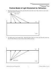
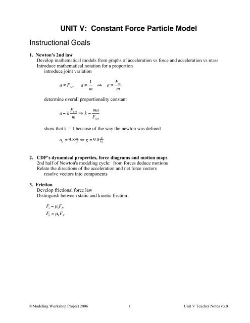
Instructional Goals
UNIT V: Constant Force Particle Model
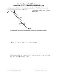
1. Newton's 2nd law
Develop mathematical models from graphs of acceleration vs force and acceleration vs mass
Introduce mathematical notation for a proportion
introduce joint variation
a "F net
a " 1 m # a " F net
m
determine overall proportionality constant
a = k F net
m " k = ma
F net
show that k = 1 because of the way the newton was defined
a g
= 9.8 m s 2
" g = 9.8 N kg
2. CDP’s dynamical properties, force diagrams and motion maps
2nd half of Newton's modeling cycle: from forces deduce motions
Relate the directions of the acceleration and net force vectors
resolve vectors into components
3. Friction
Develop frictional force law
Distinguish between static and kinetic friction
F s
= µ s
F N
F k
= µ k
F N
©Modeling Workshop Project 2006 1 Unit V Teacher Notes v3.0

Overview
In this unit, students learn the second half of Newton's Modeling Cycle:
a) from motions (read: changes in velocity) infer forces
b) from forces deduce motions
Students should be able to correctly describe the kinematic behavior of an object from the force
diagram. Typically, students are expected to be able to determine the net force, then the value of
the unknown applied force from a description of the object's kinematic behavior.
In the deployment worksheets reinforce the practice of drawing force diagrams as the first step in
preparing a solution to the problem. Make sure that these diagrams faithfully represent the
forces (long-range and contact) that act on the object. In whiteboard presentations try to induce
students to recognize multiple approaches to problems dealing with systems that consist of more
than one object.
Instructional Notes
Modified Atwood's machine lab
Apparatus
wheeled carts dynamics carts glider
wood ramps PASCO tracks airtracks
pulleys with clamps
balance for mass measurement
hangers for slotted weights (or equivalent)
spring scales (newton calibration)
photogates
ULI Timer, Logger Pro, or Data Studio software
Graphical Analysis
Pre-lab discussion
• Allow a suspended mass to tow a cart (glider) across the track; ask students to observe its motion.
We've already established that a force is required to produce an acceleration. We just haven't
quantified the relationship. Rather than brainstorming general observations, ask them to identify
other factors that might affect the acceleration of the cart. To proceed, the list must include mass,
amount of friction, and amount of force used to tow cart.
• Ask them for ideas on how to minimize the effect of friction. After some discussion, they will
hopefully come to the idea of inclining the ramp slightly to compensate for friction.
• Ask them how to measure the acceleration of the cart. While they cannot measure it directly, there
are at least two ways to do determine the acceleration. One can calculate it from rearrangement of
the kinematical model "x = 1 2 at 2 . (Note: The use of this model requires the assumption that
acceleration is constant. The rationale for such an assumption could be based on an "extra credit"
©Modeling Workshop Project 2006 2 Unit V Teacher Notes v3.0

lab.) Another method is to allow a picket fence affixed to the cart to pass through a photogate. The
slope of the velocity vs time graph yields the acceleration.
• The dependent variable is the acceleration of the cart.
• The independent variables are the mass of the cart/hanger system and the force used to pull the cart.
• Make sure to stress that the mass that is being accelerated is the total mass of the system (the cart
and hanging mass are connected, so must accelerate at the same rate).
Lab performance notes
• Use small mass hangers (e.g. 5g) and change by 10 to 20g increments.
• Increase cart mass by 0.2 - 0.5 kg increments.
• Adjust the angle of incline so that the cart can move at a constant speed with a very small initial
push.
• Convince students that they must transfer mass from the cart to the hanger in order to keep the total
mass constant when they vary the force.
• Convert the hanging mass to newtons.
• See sample graphs in Figures 1, 2, and 3.
Post-lab discussion
Figure 1 Figure 2 Figure 3
• Since the units of slope are not intuitive, focus on proportionalities.
• Discuss the combination of two proportionalities into one:
a "F net
a " 1 m # a " F net
m
• Turn the proportionality into an equation; rearrange to solve for k.
a = k F net
m " k = ma
F net
• Substitute values from regression line to solve for k. With luck, students' values should cluster
around 1.0. Now is the time to point out that the slope of force of gravity vs mass (9.8 N/kg) and the
slope of velocity vs time (9.8 m/s 2 ) have the same numerical value due to the way the newton was
defined.
©Modeling Workshop Project 2006 3 Unit V Teacher Notes v3.0

Worksheet 1
Quiz 1
Worksheet 2
Quiz 2
Friction (two approaches)
1. Demo/discussion
At this point you must decide to what depth you wish
to treat friction. If you wish to perform a
demonstration, you can use a force probe and motion
detector with a "sled" and various masses. Load
Logger Pro (MacMotion) or Data Studio software and
set up the motion detector. Calibrate the force probe,
and then re-zero it in the horizontal position.
If you steadily increase the pull on the block, the
force vs time graph should show a steady increase
until the applied force exceeds the force of static
friction and the object moves at constant velocity (use
motion detector to check this). One can obtain
the coefficients of static and kinetic friction
from the maximum and steady state values of
applied force and the normal force.
If you wish a more thorough treatment, read the
following
2. Friction Lab
Apparatus
Pre-lab discussion
• Students are asked to make observations of an object being dragged along a surface. All
observations are accepted. Friction is likely to be among the observations.
• Students are asked what affects the frictional force on the object and the surface. Ask what can be
measured or otherwise described. Things like speed, weight, area of contact, and types of surfaces
are important for students to mention.
• Guide students to the notion that it is the “support” force (normal force), rather than the force of
gravity on the object, that really is the significant factor. Showing a situation in which the two are
noticeably different can lead students to articulate this conclusion.
©Modeling Workshop Project 2006 4 Unit V Teacher Notes v3.0

• The possible difference between static and kinetic friction may be elicited by using a rather massive
box on the desk. The static frictional force may be seen to be a variable dependent on the pulling
force applied by the student, on surface area, on surface type, and on support force. Therefore, static
friction can be included in this experiment as desired. It may be desired to focus student attention on
the maximum static friction force as the significant variable which can be graphed against the
independent variables other than pulling force, because it is the single unique value that we can
associate with static friction.
• Materials available are shown to students. Force scales, objects and surfaces, mass sets, paper,
plastic, and sandpaper (to change surface types), a motor to drag objects along at various speeds, and
a photogate system to time the object as it passes, and a meter stick should be among the apparatus
available. Perhaps small pieces of wood of varying area having sandpaper, plastic, and paper
attached can ride along with the object and serve as means to change surface area.
• If felt is one of the materials used for the surface type variable, some dependence on surface area
may be observed. It appears that the increased mashing of the felt when a smaller surface area is
used produces a change in the surface character. Therefore, felt may be used as desired. It depends
on what the instructor wants the students to think about.
Lab performance notes
• A central part of this experiment will be the control of variables. Naturally, no help should be given
students regarding this other than asking them to explain what they are doing and why and to refer
lost students to others who are not so lost. The frictional force will be plotted against support force,
surface area, speed, and type of surface, so there are several variables.
• The frictional force vs surface type graph is of a different kind than previous graphs, since surface
type is not a continuous variable; a bar graph will be needed, but expect all kinds of graphs to be
made. Through discussion about the meanings of incorrectly constructed graphs, the significance of
bar graphs can become clear to students. Let them make the graphs they wish, but discuss them
carefully in the post-laboratory discussion. It can be helpful during the laboratory session to find
students making inappropriate graphs to present their results later.
Post-lab discussion
• Develop the concepts that the friction force: (a) is independent of the contact surface area; (b)
depends on the normal force (not always weight) and is different for static versus kinetic situations;
and (c) depends on the types of surfaces in contact.
• A slight dependence of frictional force on speed may be detected. Indicate that the study of velocitydependent
frictional effects is usually reserved for more advanced courses.
©Modeling Workshop Project 2006 5 Unit V Teacher Notes v3.0

• A fairly linear relationship should be apparent from the force of friction vs support force graph. The
coefficient of kinetic friction is introduced here.
• No mathematical expression will be forthcoming from the graphical model of frictional force vs
surface type. It should be concluded that each pair of surfaces will have its peculiar coefficient of
friction.
• Aim for student application of the formulas: F s ! µ s F N
F k
! µ k
F N
Worksheet 3
Worksheet 4
Unit V Test
©Modeling Workshop Project 2006 6 Unit V Teacher Notes v3.0