Cost Behaviour - CMA - Certified Management Accountants

C
Student Notes
Cost Behaviour, Part One
by John Donald, Lecturer, School of Accounting,
Economics and Finance, Deakin University, Australia
[ As a
management
accountant,
you must be
able to provide
relevant
information
on costs,
including
how they are
caused and
how they may
change
]
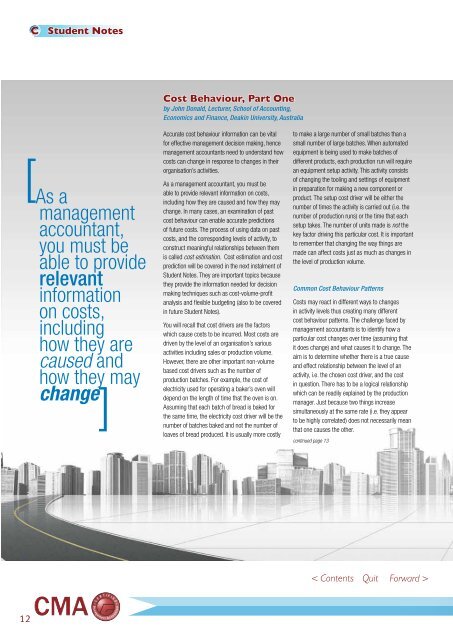
Accurate cost behaviour information can be vital
for effective management decision making, hence
management accountants need to understand how
costs can change in response to changes in their
organisation’s activities.
As a management accountant, you must be
able to provide relevant information on costs,
including how they are caused and how they may
change. In many cases, an examination of past
cost behaviour can enable accurate predictions
of future costs. The process of using data on past
costs, and the corresponding levels of activity, to
construct meaningful relationships between them
is called cost estimation. Cost estimation and cost
prediction will be covered in the next instalment of
Student Notes. They are important topics because
they provide the information needed for decision
making techniques such as cost-volume-profit
analysis and flexible budgeting (also to be covered
in future Student Notes).
You will recall that cost drivers are the factors
which cause costs to be incurred. Most costs are
driven by the level of an organisation’s various
activities including sales or production volume.
However, there are other important non-volume
based cost drivers such as the number of
production batches. For example, the cost of
electricity used for operating a baker’s oven will
depend on the length of time that the oven is on.
Assuming that each batch of bread is baked for
the same time, the electricity cost driver will be the
number of batches baked and not the number of
loaves of bread produced. It is usually more costly
to make a large number of small batches than a
small number of large batches. When automated
equipment is being used to make batches of
different products, each production run will require
an equipment setup activity. This activity consists
of changing the tooling and settings of equipment
in preparation for making a new component or
product. The setup cost driver will be either the
number of times the activity is carried out (i.e. the
number of production runs) or the time that each
setup takes. The number of units made is not the
key factor driving this particular cost. It is important
to remember that changing the way things are
made can affect costs just as much as changes in
the level of production volume.
Common Cost Behaviour Patterns
Costs may react in different ways to changes
in activity levels thus creating many different
cost behaviour patterns. The challenge faced by
management accountants is to identify how a
particular cost changes over time (assuming that
it does change) and what causes it to change. The
aim is to determine whether there is a true cause
and effect relationship between the level of an
activity, i.e. the chosen cost driver, and the cost
in question. There has to be a logical relationship
which can be readily explained by the production
manager. Just because two things increase
simultaneously at the same rate (i.e. they appear
to be highly correlated) does not necessarily mean
that one causes the other.
continued page 13
12

N TARGET
Most costs are assumed to behave in a linear
(straight line) manner but there are some costs
which behave in a curvilinear manner or which
increase in a series of steps. The assumption
that most costs are linear means that it is easy
to calculate the relevant cost function. This is a
mathematical description of how a cost changes
with changes in the level of its cost driver. A cost
function can be plotted on a graph which has the
level of the cost driver shown on the horizontal (or ‘x’
axis) and the total amount of the cost shown on the
vertical (or ‘y’ axis).
The general form of a linear cost function is simply
the formula for a straight line:
y = a + bx
where:
y = the estimated total cost amount (y is called the
dependent variable)
a = a constant which represents the component of
total cost that does not change as the level of
activity changes
b = the slope coefficient i.e. the amount by which
the total cost amount increases for a one unit
increase in the level of activity.
x = the actual (or expected future) level of activity
(x is called the independent variable)
It should be noted that assumptions about cost
behaviour are usually valid only within a restricted
range of activity called the relevant range. If the
planned level of activity falls outside the relevant or
‘normal’ range, caution is needed if past cost data
is used to predict future costs. Large increases or
decreases in output can cause costs to change
due to the addition of new production capacity (e.g.
leasing more equipment) or the reduction of existing
capacity by, for example, the elimination of unwanted
equipment and staff. We will return to this point
shortly.
The three principal categories of cost behaviour are
fixed, variable and mixed (or semi-variable).
(i) Fixed costs
These are costs that remain the same in total dollar
amount regardless of changes in the level of activity
within the relevant range. Examples would include
straight line depreciation of equipment, rent on
factory buildings, and council rates or insurance
premiums costs. The wages paid to a production
supervisor or a factory manager would also be a
fixed amount per annum provided that they are not
paid extra for working overtime. These costs (which
are really expenses) are all based on time and not on
some measure of activity or output. Because the total
amount of a fixed cost remains constant, it means
that as production volume increases fixed cost per
unit decreases.
Fixed costs are sometimes referred to as ‘capacity
costs’ as they arise from providing the facilities
needed to carry on production, for example, factory
buildings and the equipment they contain. A capital
intensive manufacturing firm such as a car maker
would have a greater proportion of fixed costs than a
labour intensive business such as a retail store.
The cost function for a fixed cost is y = a, which is
the formula for a horizontal straight line. However, the
value of ‘a’(where the total fixed cost line intersects
the y axis in Diagram 1 below) is an estimate of total
fixed costs only if the zero level of activity (shutdown)
is within the current relevant range.
Run a Better Business
13

C
Student Notes
What happens to a fixed cost if the activity level goes outside the
relevant range? It may increase or decrease in a step-wise manner as
illustrated in Diagram 2. A stepped fixed cost remains the same in
total within the various ranges of the level of an activity or output, but
the cost total increases in steps as the level of activity increases from
one range to the next.
Diagram 2 illustrates a situation where a company normally produces
between 2000 and 3000 units per annum using three leased
machines, each of which has a maximum output of 1000 units per
annum. The annual rental is $50, 000 for each machine, so the
company’s total fixed cost of operating machinery is currently $150,
000 per annum. If planned output increases or decreases from the
current level it may be possible to change the number of machines
being leased (if the lease permits this) so the total fixed cost amount
for machinery will step up or down according to which output range
the company decides to operate at.
(ii) Variable costs
A variable cost is a cost that changes, in total, in direct proportion to
changes in the level of activity. If the level of an activity doubles, and
a related cost also exactly doubles, then the cost can be classified as
a variable cost with respect to that particular activity. On a per unit
basis, however, a variable cost remains constant while the activity level
is within the relevant range. The amount of the variable cost per unit
is represented by the coefficient ‘b’ in the cost function for a variable
cost: y = bx. The value of b is the slope or gradient of the variable cost
line. Diagram 3 graphically illustrates a variable cost.
Examples of variable costs would include direct labour costs
(assuming that production workers can easily be hired or fired as
planned production goes up or down) and direct materials costs. If
the cost of direct materials is a constant $10 per production unit
then the total direct materials cost in dollars will be 10 times the
number of units produced. The total cost of fuel used by delivery
vehicles would usually vary directly with the number of kilometres
travelled. Commissions paid to sales people are normally a defined
percentage of sales dollars and so will vary in direct proportion to
sales revenue.
Notice that the cost line in Diagram 3 starts at the origin, which is
the point where the x and y axes intersect. At zero units produced,
total variable cost is also zero, while the uniform slope of the cost
line reflects the constant variable cost per unit within the relevant
range. If variable cost per unit does change at certain levels of
activity, the variable cost line will be made up of a number of
short straight segments each covering a certain range of activity
14

N TARGET
Cost
Cost
Cost
Cost
TFC
TFC
Cost
Co
TFC
TFC
Production Volume Production (units per Volume annum) (units per annum)
Diagram 1: A Fixed Cost Diagram 1: A Fixed Cost
Production Volume (units Production per annum) Volume (units per annum)
Diagram 2: A Stepped Fixed Diagram Cost 2: A Stepped Fixed Cost
Production Volume (uni P
Diagram 3: A Variab
Cost
Cost
TVC
TVC
Cost
Cost
TC
TC
Production Volume Production (units Volume per annum) (units per annum)
Diagram 3: A Variable Diagram Cost 3: A Variable Cost
Production Volume Production (units Volume per annum) (units per annum)
Diagram 4: A Mixed Diagram (or Semi-Variable) 4: A Mixed (or Semi-Variable) Cost
Cost
and each having a different slope. The variable cost line will, if the
ranges are small enough, take on a curvilinear shape. If variable cost
per unit steadily increases as the level of activity increases, the cost
line will curve upwards i.e. its slope will become steeper. For example,
the cost of electricity per kilowatt-hour may increase each time that
total electricity consumption for a period (in kilowatt-hours) passes
a certain level. When the level of activity rises and causes electricity
consumption to reach a cost change point, the slope of the electricity
cost line will increase for the next range of activity.
(iii) Mixed costs
The costs considered so far have been either completely fixed or completely
variable. However, there are some costs, called mixed or semi-variable costs,
which have both fixed and variable components as shown in Diagram 4.
For example, an electricity bill will usually include a fixed supply charge for
a certain time period as well as a charge for the total amount of electricity
consumed during that period. Even if production lines had been completely
shut down for the whole of the billing period, and no electricity had been
used, the fixed supply charge must be paid. This is the minimum cost
of keeping electric power available for the factory. It represents the fixed
component of total electricity cost i.e. the amount of cost where the cost
line in Diagram 4 intersects the vertical (y) axis. It is also the value of the
constant ‘a’ in the cost function for a mixed cost: y = a + bx. As previously
mentioned, b is the variable (or incremental) cost per unit of activity.
Mixed costs are usually reported in total in the accounting records. How
much of the cost is fixed and how much is variable is sometimes unknown
and must be estimated. The ways that this can be done will be explained in
the next instalment of Student Notes.
Why is it important to know which costs are fixed and which are variable?
This information is useful for management decision making, for instance,
when considering whether to sell a certain quantity of output to a special
customer at a unit price which is less than the full production cost per unit.
An understanding of the costs that will increase with the level of activity,
compared to those costs that will remain constant over the relevant range
of activity, also assists managers in determining how cost reductions will
add to the firm’s profitability. But beware; fixed costs per unit should be
used carefully for internal decision making because they will vary as output
varies. If fixed cost per unit decreases, it simply means that total fixed
costs are being spread over more units and not that total fixed costs have
changed. A final, but important, point: determining whether a cost is fixed
or variable depends on the time horizon. The longer the time period, the
more likely it is that a cost will be variable. The so-called ‘short run’ is a
period of time for which at least one cost remains fixed. In the long run, all
costs are variable.
Run a Better Business
15