Statistical Estimation of Refractivity from Radar Sea Clutter
Statistical Estimation of Refractivity from Radar Sea Clutter
Statistical Estimation of Refractivity from Radar Sea Clutter

Create successful ePaper yourself
Turn your PDF publications into a flip-book with our unique Google optimized e-Paper software.
<strong>Statistical</strong> <strong>Estimation</strong> <strong>of</strong> <strong>Refractivity</strong> <strong>from</strong> <strong>Radar</strong><br />
<strong>Sea</strong> <strong>Clutter</strong><br />
Caglar Yardim, Peter Gerst<strong>of</strong>t, William S. Hodgkiss<br />
University <strong>of</strong> California, San Diego<br />
La Jolla, CA 92093–0238, USA<br />
email: cyardim@ucsd.edu, gerst<strong>of</strong>t@ucsd.edu,<br />
whodgkiss@ucsd.edu<br />
Ted Rogers<br />
Space and Naval Warfare Systems Center<br />
San Diego, CA 92152, USA<br />
email: trogers@spawar.navy.mil<br />
Abstract— This paper summarizes current developments in<br />
the refractivity <strong>from</strong> clutter (RFC) techniques and describes<br />
the global parametrization approach in estimation <strong>of</strong> the lower<br />
atmospheric electromagnetic sea ducts. RFC uses radar clutter to<br />
gather information about the environment the radar is operating<br />
in. Range and height dependent atmospheric index <strong>of</strong> refraction<br />
(M-pr<strong>of</strong>ile) is statistically estimated <strong>from</strong> the sea-surface reflected<br />
radar clutter. These environmental statistics can then be used<br />
to predict the radar performance by taking multidimensional<br />
integrals <strong>of</strong> the posterior probability density.<br />
All <strong>of</strong> the following methods use a Bayesian framework and<br />
use split-step fast Fourier transform based parabolic equation<br />
approximation to the wave equation as the propagation model.<br />
Environmental parameters are inverted using genetic algorithms,<br />
Markov chain Monte Carlo samplers, and a hybrid genetic<br />
algorithm - Markov chain Monte Carlo technique. The methods<br />
are compared with respect to their estimated maximum a<br />
posteriori accuracy, speed and ability to sample correctly <strong>from</strong><br />
posterior density. The inversion algorithms are implemented on<br />
S-band radar sea-clutter data <strong>from</strong> 1998 Wallops Island, Virginia<br />
experiment. Reference data are measured as range-dependent<br />
refractivity pr<strong>of</strong>iles obtained with a helicopter. The inversions are<br />
assessed by comparing the propagation predicted <strong>from</strong> the radarinferred<br />
refractivity pr<strong>of</strong>iles and <strong>from</strong> the helicopter pr<strong>of</strong>iles.<br />
I. INTRODUCTION<br />
Non-standard electromagnetic propagation due to formation<br />
<strong>of</strong> lower atmospheric sea ducts is a common occurrence in<br />
maritime radar applications. Under these conditions, some<br />
fundamental system parameters <strong>of</strong> a sea-borne radar can significantly<br />
deviate <strong>from</strong> their original values specified assuming<br />
standard-air (0.118 M-units/m) conditions. These include the<br />
variation in the maximum operational range, creation <strong>of</strong> regions<br />
where the radar is practically blind (radar holes), and<br />
increased sea surface clutter (1). Therefore, it is important<br />
to predict the real-time environment the radar is operating in<br />
so that the radar operator will at least know the true system<br />
limitations and in some cases even compensate for it.<br />
Evaporation and surface-based ducts are associated with<br />
increased sea clutter due to the heavy interaction between the<br />
sea surface and the electromagnetic signal trapped within the<br />
duct. However, this unwanted clutter is a rich source <strong>of</strong> information<br />
about the environment and can be used to determine the<br />
local atmospheric conditions. This can be a valuable addition<br />
to other more conventional techniques such as radiosondes,<br />
rocketsondes, microwave refractometers and meteorological<br />
−250<br />
−200<br />
−150<br />
−100<br />
−50<br />
0<br />
50<br />
100<br />
150<br />
200<br />
Reflectivity image: April 02, 1998 Map # 040298−12 18:00:00.3<br />
200 km<br />
150 km<br />
100 km<br />
50 km<br />
250<br />
−250 −200 −150 −100 −50 0 50 100 150 200 250<br />
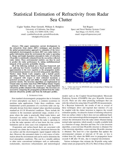
Fig. 1. <strong>Clutter</strong> map <strong>from</strong> the SPANDAR radar corresponding to Wallops run<br />
12 with 0 o elevation angle.<br />
models such as the Coupled Ocean/Atmospheric Mesoscale<br />
Prediction System (COAMPS) that give M-pr<strong>of</strong>ile forecasts<br />
[1]–[4]. There are also other promising techniques that can<br />
refer the refractivity using lidar [5] and GPS [6] measurements.<br />
In a Bayesian framework, the results <strong>of</strong> one or several <strong>of</strong><br />
these techniques above and regional duct statistics [7] can<br />
be coupled with the clutter inversion to improve the overall<br />
estimation quality. An attractive feature <strong>of</strong> inferring refractivity<br />
<strong>from</strong> sea surface clutter is that it does not use additional hardware<br />
or extra meteorological/electromagnetic measurements. It<br />
extracts the information <strong>from</strong> the radar clutter obtained during<br />
normal radar operation, which usually is readily available both<br />
as a function <strong>of</strong> range, direction and time. For a fast inversion<br />
algorithm, a near-real-time M-pr<strong>of</strong>ile structure is obtained. For<br />
a fast inversion algorithm, a near-real-time M-pr<strong>of</strong>ile structure<br />
is obtained. The need for a fast algorithm that updates the<br />
environmental estimates at intervals <strong>of</strong> 30 min. or less is<br />
evident <strong>from</strong> [8], where the RMS error in propagation factor<br />
exceeds 6 dB after 30 min., due to temporal decorrelation.<br />
Various techniques that estimate the M-pr<strong>of</strong>ile using radar<br />
clutter return are proposed by [9]–[15]. Most <strong>of</strong> these refractiv-<br />
40<br />
35<br />
30<br />
25<br />
20<br />
15<br />
10<br />
5<br />
0
ity <strong>from</strong> clutter (RFC) techniques use an electromagnetic fast<br />
Fourier transform (FFT) split-step parabolic equation (SSPE)<br />
approximation to the wave equation [16], [17], whereas some<br />
also make use <strong>of</strong> ray-tracing techniques. While [9] exclusively<br />
concerns evaporation duct estimation, other techniques are<br />
applicable to both evaporation, surface-based and mixed type<br />
<strong>of</strong> ducts that contain both an evaporation section and an<br />
surface-based type inversion layer. [15] exploits the inherent<br />
Markovian structure <strong>of</strong> the FFT parabolic equation approximation<br />
and uses a particle filtering approach, whereas [12] uses<br />
rank correlation with ray tracing to estimate the M-pr<strong>of</strong>ile.<br />
In contrast, [10], [11], [14] and [18] use global parameterization<br />
within a Bayesian framework. Since the unknown model<br />
parameters are defined as random variables in a Bayesian<br />
framework, the inversion results will be in terms <strong>of</strong> the means,<br />
variances and marginal, as well as the n-dimensional joint<br />
posterior probability distributions, where n is the number <strong>of</strong><br />
unknown duct parameters. This gives the user not only the<br />
ability to obtain the maximum a posteriori (MAP) solution,<br />
but also the prospect <strong>of</strong> performing statistical analysis on the<br />
inversion results and the means to convert these environmental<br />
statistics into radar performance statistics. These statistical<br />
calculations can be performed by taking multi-dimensional<br />
integrals <strong>of</strong> the joint PPD. [10] uses genetic algorithms to<br />
estimate the MAP solution. However, no statistical analysis is<br />
performed since classical GA is not suitable for the necessary<br />
integral calculations. While [11] uses importance sampling,<br />
[14] uses Markov chain Monte Carlo (MCMC) samplers to<br />
perform the MC integration [19], [20]. Although they provide<br />
the means to quantify the impact <strong>of</strong> uncertainty in the estimated<br />
duct parameters, they require large numbers <strong>of</strong> forward<br />
model runs and hence they lack the speed to be near-real-time<br />
methods and are not suitable for models with large numbers<br />
<strong>of</strong> unknowns.<br />
A hybrid GA-MCMC method based on the nearest neighborhood<br />
algorithm (NA) [21] has been implemented in [18].<br />
It can be classified as an improved GA method, which<br />
improves integral calculation accuracy through hybridization<br />
with a MCMC sampler. Since the number <strong>of</strong> forward model<br />
samples is based on GA, it requires fewer samples than a<br />
MCMC, enabling inversion <strong>of</strong> atmospheric models with higher<br />
complexity with larger number <strong>of</strong> unknowns.<br />
II. THEORY<br />
To formulate the problem, a Bayesian framework is adopted,<br />
where the M-pr<strong>of</strong>ile model and the radar measured sea-surface<br />
clutter data are denoted by the vectors m and d, respectively.<br />
An electromagnetic FFT-SSPE is used to propagate the field in<br />
an environment given by m and obtain synthetic clutter returns<br />
f(m). Since the unknown environmental parameters m are<br />
assumed to be random variables, the solution to the inversion is<br />
given by their joint posterior probability distribution function<br />
(PPD or p(m|d)). More theory can be found in [10], [11],<br />
[14], [18], each one corresponding for one <strong>of</strong> the methods<br />
summarized here. Bayes’ formula can be used to write the<br />
Environmental<br />
domain<br />
m<br />
Data domain<br />
d<br />
Usage domain<br />
Utility u<br />
Fig. 2. An observation d is mapped into a distribution <strong>of</strong> environmental<br />
parameters m that potentially could have generated it. The environmental<br />
parameters are then mapped into the usage domain u.<br />
PPD as<br />
p(m|d) =<br />
L(m)p(m)<br />
∫m ′ L(m′ )p(m ′ )dm ′ , (1)<br />
where p(m) is the prior probability distribution function<br />
(pdf) <strong>of</strong> the parameters. Any information obtained <strong>from</strong> other<br />
methods and regional duct statistics can be incorporated in this<br />
step as a prior belief. Since this paper investigates the ability to<br />
infer M-pr<strong>of</strong>iles using RFC, a uniform prior is used. However,<br />
it is possible to include statistical meteorological priors <strong>from</strong><br />
studies such as [7], for some <strong>of</strong> the parameters (e.g. the duct<br />
height).<br />
Assuming a zero-mean Gaussian error between the measured<br />
and modeled clutter, the likelihood function is given by<br />
L(m) = (2π) −NR/2 |C d | −1/2 (2)<br />
× exp<br />
[− (d − f(m))T C −1<br />
]<br />
d<br />
(d − f(m))<br />
,<br />
2<br />
where C d is the data error covariance matrix, (·) T is the<br />
transpose and N R is the number <strong>of</strong> range points used (length<br />
<strong>of</strong> the data vector, d). Further simplification can be achieved<br />
by assuming that the errors are spatially uncorrelated with<br />
identical distribution for each data point forming the vector<br />
d. For this case, C d = νI, where ν is the variance and I the<br />
identity matrix. Then the equation can be simplified to<br />
p(m|d) ∝<br />
[ ] NR/2<br />
N R<br />
p(m)<br />
2πeφ(m)<br />
(3)<br />
φ(m) = (d − f(m)) T (d − f(m)) . (4)<br />
Having defined the posterior density, any statistical information<br />
about the unknown environmental and radar parameters<br />
can now be calculated by taking these multi-dimensional<br />
integrals:<br />
∫ ∫<br />
µ i = ... m ′ ip(m ′ |d)dm ′ (5)<br />
∫ ∫<br />
σi 2 = ... (m ′ i − µ i ) 2 p(m ′ |d)dm ′ (6)<br />
∫ ∫<br />
p(m i |d) = ... δ(m ′ i − m i )p(m ′ |d)dm ′ (7)<br />
where µ i , σ 2 i ,p(m i|d) are posterior means (Bayesian minimum<br />
mean square error (MMSE) estimate), variances, and<br />
marginal PPD’s <strong>of</strong> M-pr<strong>of</strong>ile parameters.
Probability distributions <strong>of</strong> parameters <strong>of</strong> interest to a radar<br />
operator are calculated in a similar fashion [11]. Assume that u<br />
is such a parameter-<strong>of</strong>-interest (e.g. propagation factor), which<br />
naturally is some function u =g(m) <strong>of</strong> the radar environment<br />
m (Fig. 2). A statistical analysis <strong>of</strong> u can be carried out by<br />
computing the following MC integration<br />
∫ ∫<br />
p(u|d) = ... δ(u − g(m ′ ))p(m ′ |d)dm ′ . (8)<br />
III. SELECTION OF SAMPLER/OPTIMIZER<br />
The question is about how to efficiently compute these<br />
multi-dimensional integrals and MAP solutions. The following<br />
list summarizes the techniques that have been used in previous<br />
work:<br />
• Genetic algorithms (GA) is used in [10] to successfully<br />
compute the MAP solution. Among all the following<br />
methods GA is the fastest method in obtaining the MAP.<br />
However, it fails to obtain PPD so no integral calculation<br />
can be performed.<br />
• Importance sampling (IS) is used in [11]. This allows<br />
computation <strong>of</strong> the necessary posterior integrals without<br />
needing to sample <strong>from</strong> the PPD. It is accurate as long as<br />
the prior is not significantly different <strong>from</strong> the PPD since<br />
it gathers the samples necessary for MC integration <strong>from</strong><br />
the prior.<br />
• Markov chain Monte Carlo (MCMC) samplers are used in<br />
[14]. MCMC allows sampling directly <strong>from</strong> the PPD and<br />
hence provides the best estimates <strong>of</strong> the integral required.<br />
However it requires a lot <strong>of</strong> samples to converge.<br />
• Hybrid GA–MCMC method is used in [18]. This technique<br />
is a hybrid between the fastest and the most<br />
accurate technique, trying to get reasonably integral calculations<br />
using much less forward model runs, typically<br />
on the order <strong>of</strong> a GA run. It uses Voronoi decomposition<br />
to approximate the PPD using a typical GA run and then<br />
run a MCMC on this approximate PPD minimizing the<br />
parabolic equation calculations.<br />
The hybrid method can be summarized by the following<br />
steps:<br />
1) GA: Run a classical GA, minimizing the misfit φ(m),<br />
save all the populations (sampled model vectors) and<br />
their likelihood values. MAP solution is obtained as the<br />
best fit model vector.<br />
2) Voronoi Decomposition and Approximate PPD: Using<br />
the GA samples {m i } and their corresponding p(m i |d)<br />
construct the Voronoi cell structure and create the approximate<br />
PPD, ̂p(m|d).<br />
3) Gibbs Resampling: Run a fast GS on the approximate<br />
PPD. No forward modeling is needed.<br />
4) MC Integral Calculations: Calculate the Bayesian minimum<br />
mean square estimate (MMSE), variance and posterior<br />
distributions <strong>of</strong> desired environmental parameters,<br />
statistics for the end-user parameters, such as propagation<br />
loss L, propagation factor F, coverage diagrams,<br />
statistical radar performance prediction, such as the<br />
Fig. 3.<br />
inversion<br />
slope, c2<br />
base<br />
slope, c 1<br />
top layer slope<br />
0.118 M-units/m<br />
inversion thickness, h<br />
base height, h 1<br />
2<br />
Four-parameter range-independent tri-linear M-pr<strong>of</strong>ile.<br />
probability <strong>of</strong> detection and false alarm using (5) – (7),<br />
and (8) using MC integration.<br />
IV. EXAMPLES<br />
Three examples are presented in this section. The first shows<br />
how to estimate MC integral using the importance sampling,<br />
the second compares GA, MCMC and the hybrid methods and<br />
the last one analyzes a range-dependent pr<strong>of</strong>ile with a high<br />
number <strong>of</strong> parameters using the hybrid method.<br />
The first example is created using a range-dependent 8<br />
parameter surface-based duct formed using 2 tri-linear M-<br />
pr<strong>of</strong>iles at 0 and 100 km, where a typical tri-linear pr<strong>of</strong>ile<br />
is shown in Fig. 3. It is taken <strong>from</strong> [11]. The unknown model<br />
parameters are the slope and height <strong>of</strong> the base layer (c 1 and<br />
h 1 ) and the slope and thickness <strong>of</strong> the inversion layer (c 2 and<br />
h 2 ). Since the RFC is insensitive to the M-pr<strong>of</strong>ile parameters<br />
above the duct, the top layer slope corresponds to standard<br />
atmosphere. The data are generated based on the helicopter<br />
measured range-dependent refractivity pr<strong>of</strong>ile (run 7) for the<br />
Wallops 98 experiment. Then samples are drawn <strong>from</strong> the prior<br />
density given in Fig. 4 and their likelihood are computed using<br />
(2). Any required parameter can now be computed by using<br />
these likelihood values as appropriate weight factors in integral<br />
calculations. 1-D and 2-D PPD estimate is given in Fig. 5.<br />
Note that any integral using importance sampling will be less<br />
accurate if prior is too different with respect to the PPD such<br />
as the third parameter (slope 1) in this examples.<br />
The second example is [18] a 4 parameter surface-based<br />
duct. This example compares GA, MCMC and the hybrid<br />
methods in terms <strong>of</strong> their computational complexity, MAP<br />
accuracy, and PPD estimation accuracy. It computes the true<br />
values using exhaustive search to provide a benchmark. 1-<br />
D marginal model parameter PPD’s are given in Fig. 6 for<br />
(a) exhaustive search, (b) Metropolis-Hastings sampler (conventional<br />
MCMC), (c) pure GA, and (d) hybrid GA-MCMC<br />
method, respectively. Exhaustive search results are assumed<br />
to have a dense enough grid to give the true distributions<br />
and will be used as the benchmark. As expected, the Gibbs<br />
sampler results are close to the true distribution but requires<br />
70x10 3 (70k) samples to converge. The GA uses 15k samples<br />
(5k is enough to get the MAP solution). The distributions are<br />
clearly not accurate, however, as a global optimizer it does
0.4<br />
0.2<br />
400<br />
200<br />
400<br />
200<br />
400<br />
200<br />
0.01<br />
0.3<br />
0.2<br />
0.1<br />
400<br />
200<br />
400<br />
200<br />
400<br />
200<br />
x 10 −3<br />
15<br />
10<br />
5<br />
0<br />
0 200 400<br />
Baseheight 1 (m)<br />
0<br />
0 200 400<br />
0.4<br />
0<br />
−1 −0.5 0<br />
400<br />
0<br />
−1 −0.5 0<br />
400<br />
0<br />
0<br />
0 200 400<br />
Baseheight 1 (m)<br />
0<br />
0 200 400<br />
0.3<br />
0<br />
−1 −0.5 0<br />
400<br />
0<br />
−1 −0.5 0<br />
400<br />
0.2<br />
200<br />
200<br />
0.2<br />
0.1<br />
200<br />
200<br />
0<br />
0 200 400<br />
Baseheight 2 (m)<br />
0<br />
−1 −0.5 0<br />
0.4<br />
0<br />
−1 −0.5 0<br />
0<br />
0<br />
0 200 400<br />
Baseheight 2 (m)<br />
0<br />
−1 −0.5 0<br />
0.3<br />
0<br />
−1 −0.5 0<br />
0<br />
0.2<br />
−0.5<br />
0.2<br />
0.1<br />
−0.5<br />
0<br />
−1 −0.5 0<br />
Slope 1 (M/m)<br />
−1<br />
−1 −0.5 0<br />
0.4<br />
0<br />
−1 −0.5 0<br />
Slope 1 (M/m)<br />
−1<br />
−1 −0.5 0<br />
0.3<br />
0.2<br />
0.2<br />
0.1<br />
0<br />
−1 −0.5 0<br />
Slope 2 (M/m)<br />
0<br />
−1 −0.5 0<br />
Slope 2 (M/m)<br />
Fig. 4. Prior probability distribution for the base height and slope at 0<br />
and 100 km range. Along the diagonal the marginal for each parameter is<br />
plotted, and above the diagonal show the 2D marginals (red indicates higher<br />
probability). The distributions below the diagonal are symmetric with those<br />
above.<br />
Fig. 5. Posterior probability distribution for the base height and slope at<br />
0 and 100 km range. Along the diagonal the marginal for each parameter is<br />
plotted, and above the diagonal show the 2D marginals (red indicates higher<br />
probability). The distributions below the diagonal are symmetric with those<br />
above.<br />
its job <strong>of</strong> minimizing φ(m) and obtaining MAP very fast.<br />
The GA sample histograms presented here are not unique.<br />
Every GA run will result in a different set <strong>of</strong> curves, without<br />
any specific sampling density p s (m|d). The hybrid method<br />
actually uses the 15k GA samples obtained in (c) to perform<br />
the Voronoi decomposition. When a fast Gibbs resampling is<br />
performed on the approximate PPD, results comparable to the<br />
conventional MCMC solution is obtained. A Gibbs resampling<br />
<strong>of</strong> just 20k samples is sufficient to calculate the MC integral<br />
accurately (40k is used in (d)). It should be noted that (d) is<br />
extracted using the forward model samples obtained in (c).<br />
All information about the search space comes <strong>from</strong> the GA<br />
samples and the hybrid method makes the information hidden<br />
in the GA set available for MC integration through Voronoi<br />
decomposition.<br />
The final example is taken <strong>from</strong> [18]. To further demonstrate<br />
the capabilities and limitations <strong>of</strong> the hybrid method, a<br />
range-dependent environmental model comprising <strong>of</strong> sixteen<br />
parameters is employed during the inversion <strong>of</strong> the 1998<br />
Wallops island experiment data. A range dependent inversion<br />
is achieved by defining vertical, four-parameter tri-linear M-<br />
pr<strong>of</strong>iles at certain ranges (0, 20, 40, and 60 km) and linearly<br />
interpolating the parameters in between. Slopes for both the<br />
first and the second layers can be negative and positive to give<br />
more flexibility in the modeling. Hence, they are only referred<br />
to by their layer numbers. Layer slopes at different ranges can<br />
vary independent <strong>of</strong> each other. On the contrary, a Markovian<br />
structure is used for the layer heights with a maximum <strong>of</strong> 30<br />
m variation relative to the height value at the previous range.<br />
The height values except for the first pr<strong>of</strong>ile are difference<br />
in meters between the layer thicknesses <strong>of</strong> two consecutive<br />
pr<strong>of</strong>iles, so they can be ±30 m.<br />
(a) 5<br />
(b)<br />
(c)<br />
(d)<br />
c 1<br />
0<br />
0.1 0.15 0.2<br />
5<br />
0<br />
0.1 0.15 0.2<br />
10<br />
5<br />
0<br />
0.1 0.15 0.2<br />
5<br />
0<br />
0.1 0.15 0.2<br />
M-units/m<br />
5<br />
c h h 2<br />
2<br />
5<br />
0<br />
38<br />
1<br />
40 42<br />
5<br />
0<br />
20 40<br />
5<br />
5<br />
0<br />
-2.6 -2.4 -2.2<br />
5<br />
0<br />
-2.6 -2.4 -2.2<br />
10<br />
5<br />
0<br />
-2.6 -2.4 -2.2<br />
5<br />
0<br />
-2.6 -2.4 -2.2<br />
M-units/m<br />
0<br />
38 40 42<br />
0<br />
10<br />
10<br />
5<br />
5<br />
0<br />
38 40 42<br />
0<br />
5<br />
5<br />
0<br />
38 40 42<br />
m<br />
0<br />
20 40<br />
20 40<br />
20 40<br />
m<br />
Fig. 6. Marginal posterior probability distributions for the synthetic test case.<br />
Vertical lines show the true values <strong>of</strong> the parameters. (a) Exhaustive search,<br />
(b) Metropolis sampler (MCMC), (c) GA, and (d) hybrid GA-MCMC using<br />
15k GA and 40k Gibbs samples.<br />
Only 13 out <strong>of</strong> 16 parameters are given in Fig. 7(a). The<br />
height parameters <strong>of</strong> the second layers m 8 ,m 12 , and m 16 are<br />
omitted, as they are not important. Since clutter is mostly due<br />
to the EM signal trapped inside the duct, it mostly contains<br />
information about the parameters inside the duct, making<br />
the second layer heights poorly determined except for very<br />
close ranges. To demonstrate this, normalized error function<br />
φ(m)/φ(m MAP ) for various conditional planes are given in<br />
Fig. 7(b). These curves are obtained by fixing other parameters<br />
to their MAP values and calculating φ(m) while varying only<br />
two parameters at a time. Except for the bottom plots all the<br />
plots show quickly varying complex patterns whereas the last<br />
ones are flat since the horizontal axis for these is either m 8 ,
Fig. 7. Marginal and conditional distributions. (a)1-D (diagonal) and 2-D (upper diagonal) posterior probability distributions in terms <strong>of</strong> percent HPD, for<br />
the range-dependent SPANDAR data inversion. 13 parameters (m 1−7 , m 9−11 , m 13−15 ) out <strong>of</strong> 16 are given . Vertical lines in the 1-D plots show the GA<br />
MAP solution. (b) Normalized error function for various conditional planes. Each 2-D plot is obtained by fixing the other 14 parameters to their MAP values.<br />
m 12 , or m 16 (second layer heights). Some plots such as m 1 vs.<br />
m 12 have zero likelihood regions since the height parameters<br />
which are ∆h at 20, 40, and 60 km cannot be less than values<br />
that would make the actual layer thickness negative.<br />
The environmental statistics can be projected into statistics<br />
for user parameters (see Section II). One typical parameter <strong>of</strong><br />
interest to an end-user is the propagation factor F. The results<br />
in Fig. 8 are obtained <strong>from</strong> the parameter PPD in Fig. 7. It<br />
shows the PPD for F at ranges (a) 18, (b) 40, and (c) 60 km.<br />
Contour plots show the PPD <strong>of</strong> F for height values between<br />
0–200 m, with the MAP solution (dashed white). Horizontal<br />
lines represent the three altitudes analyzed in detail in the small<br />
plots shown next to the color plots. Comparison <strong>of</strong> plots at<br />
the same range and different altitudes reveals some important<br />
aspects <strong>of</strong> RFC.<br />
First, the propagation factor PPDs inside the duct (at 20<br />
m) are sharper than those outside the duct (100 and 180<br />
m). This is expected since we used the sea clutter which is<br />
usually affected only by the lower portions <strong>of</strong> the atmosphere<br />
to infer the environment. The PPDs do also become flatter<br />
with increasing range. Note how the error made by using<br />
the standard atmospheric assumption (black dashed lines)<br />
increases with range, especially inside the duct. At [H, R] =<br />
[20 m, 18 km] all three curves (MAP, helicopter pr<strong>of</strong>ile, and<br />
standard atmosphere) are almost identical whereas standard<br />
atmospheric assumption leads to more than 40 dB error for [H,<br />
R] = [20 m, 60 km] while MAP and helicopter pr<strong>of</strong>ile comply<br />
with the underlying PPD. Finally, the difference between the<br />
helicopter pr<strong>of</strong>ile and MAP tends to be larger outside the duct.<br />
V. CONCLUSION<br />
Various RFC methods has been summarized. These methods<br />
have been used for statistical sea-borne radar performance estimation<br />
under non-standard propagation conditions. <strong>Statistical</strong><br />
refractivity-<strong>from</strong>-clutter (RFC) inversion is used to gather information<br />
about the environment, such as the range-dependent<br />
vertical structure <strong>of</strong> the atmospheric index <strong>of</strong> refraction, and<br />
then these environmental uncertainties are used to estimate<br />
parameters-<strong>of</strong>-interest to be used by the radar operator.<br />
As a forward model, a fast Fourier transform split-step<br />
parabolic equation (FFT-SSPE) approximation to the wave
200<br />
180<br />
160<br />
R = 18 km<br />
95<br />
90<br />
80<br />
70<br />
50<br />
40<br />
20<br />
H = 10 m<br />
R = 40 km<br />
H = 10 m<br />
R = 60 km<br />
H = 10 m<br />
140<br />
−40 −20 0 20<br />
−40 −20 0 20<br />
−40 −20 0 20<br />
H = 50 m<br />
H = 50 m<br />
H = 50 m<br />
120<br />
height (m)<br />
100<br />
80<br />
−40 −20 0 20<br />
−40 −20 0 20<br />
−40 −20 0 20<br />
60<br />
H = 90 m<br />
H = 90 m<br />
H = 90 m<br />
40<br />
20<br />
−40 −20 0 20 −40 −20 0 20<br />
Propagation Factor, F (dB) F (dB)<br />
−40 −20 0 20<br />
Propagation Factor, F (dB)<br />
−40 −20 0 20<br />
F (dB)<br />
−40 −20 0 20<br />
Propagation Factor, F (dB)<br />
−40 −20 0 20<br />
F (dB)<br />
Fig. 8. Posterior probability densities for propagation factor F at three different ranges: (a) 18, (b) 40, and (c) 60 km. Color plots show the PPD <strong>of</strong> F for<br />
height values between 0 m and 200 m in terms <strong>of</strong> percent HPD, with the MAP solution (dashed white). Horizontal lines represent the three altitudes analyzed<br />
in detail in the small plots shown next to the color plots at heights 180, 100, and 20 m, respectively <strong>from</strong> top to bottom. Vertical lines in the small plots<br />
represent the values <strong>of</strong> F at the corresponding height and range for the MAP solution (blue line with circles), helicopter measurement (red), and standard<br />
atmospheric assumption (black).<br />
equation was used to propagate the electromagnetic signal in<br />
complex environments. The hybrid method uses fewer forward<br />
model calculations than a classical MCMC while obtaining<br />
more accurate distributions than GA. This enables inclusion <strong>of</strong><br />
more unknown parameters and range-dependent atmospheric<br />
models. The capabilities <strong>of</strong> the technique were illustrated for<br />
a sixteen dimensional range-dependent inversion.<br />
VI. ACKNOWLEDGMENT<br />
This work was supported by the Office <strong>of</strong> Naval Research<br />
under grant N00014-05-1-0369.<br />
REFERENCES<br />
[1] J. R. Rowland and S. M. Babin, “Fine-scale measurements <strong>of</strong> microwave<br />
pr<strong>of</strong>iles with helicopter and low cost rocket probes,” Johns Hopkins APL<br />
Tech. Dig., vol. 8 (4), pp. 413–417, 1987.<br />
[2] E. R. Thews, “Timely prediction <strong>of</strong> low-altitude radar performance in<br />
operational environments using in situ atmospheric refractivity data,”<br />
IEE Proc., vol. 137 (F-2), pp. 89–94, 1990.<br />
[3] R. M. Hodur, “The naval research laboratory’s coupled<br />
ocean/atmosphere mesoscale prediction system (COAMPS),” Monthly<br />
Weather Review, vol. 125(7), pp. 1414–1430, 1996.<br />
[4] M.I.Skolnik,Introduction to <strong>Radar</strong> Systems, 3rd ed. New York:<br />
McGraw–Hill, 2001.<br />
[5] A. Willitsford and C. R. Philbrick, “Lidar description <strong>of</strong> the evaporative<br />
duct in ocean environments,” vol. 5885. Proceedings <strong>of</strong> SPIE,<br />
Bellingham, WA, September 2005.<br />
[6] A. R. Lowry, C. Rocken, S. V. Sokolovskiy, and K. D. Anderson, “Vertical<br />
pr<strong>of</strong>iling <strong>of</strong> atmospheric refractivity <strong>from</strong> ground-based GPS,” Radio<br />
Science, vol. 37(3), pp. 1041–1059, 2002, doi:10.1029/2000RS002565.<br />
[7] S. M. Babin, “Surface duct height distrubutions for Wallops island,<br />
Virginia, 1985–1994,” Journal <strong>of</strong> Applied Meteorology, vol. 35 (1), pp.<br />
86–93, 1996.<br />
[8] L. T. Rogers, “Effects <strong>of</strong> variability <strong>of</strong> atmospheric refractivity on<br />
propagation estimates,” IEEE Trans. Antennas Propagat., vol.44(4),<br />
pp. 460–465, 1996.<br />
[9] L. T. Rogers, C. P. Hattan, and J. K. Stapleton, “Estimating evaporation<br />
duct heights <strong>from</strong> radar sea echo,” Radio Science, vol. 35 (4), pp. 955–<br />
966, 2000, doi:10.1029/1999RS002275.<br />
[10] P. Gerst<strong>of</strong>t, L. T. Rogers, J. Krolik, and W. S. Hodgkiss, “Inversion for<br />
refractivity parameters <strong>from</strong> radar sea clutter,” Radio Science, vol.38<br />
(3), pp. 1–22, 2003, doi:10.1029/2002RS002640.<br />
[11] P. Gerst<strong>of</strong>t, W. S. Hodgkiss, L. T. Rogers, and M. Jablecki, “Probability<br />
distribution <strong>of</strong> low altitude propagation loss <strong>from</strong> radar sea-clutter data,”<br />
Radio Science, vol. 39, pp. 1–9, 2004, doi:10.1029/2004RS003077.<br />
[12] A. Barrios, “<strong>Estimation</strong> <strong>of</strong> surface-based duct parameters <strong>from</strong> surface<br />
clutter using a ray trace approach,” Radio Science, vol. 39 RS6013, pp.<br />
1–15, 2004, doi:10.1029/2003RS002930.<br />
[13] L. T. Rogers, M. Jablecki, and P. Gerst<strong>of</strong>t, “Posterior distributions <strong>of</strong><br />
a statistic <strong>of</strong> propagation loss inferred <strong>from</strong> radar sea clutter,” Radio<br />
Science, vol. 40 (6), pp. 1–14, 2005, doi:10.1029/2004RS003112.<br />
[14] C. Yardim, P. Gerst<strong>of</strong>t, and W. S. Hodgkiss, “<strong>Estimation</strong> <strong>of</strong> radio<br />
refractivity <strong>from</strong> radar clutter using Bayesian Monte Carlo analysis,”<br />
IEEE Trans. Antennas Propagat., vol. 54(4), pp. 1318–1327, 2006.<br />
[15] S. Vasudevan, R. Anderson, S. Kraut, P. Gerst<strong>of</strong>t, L. Rogers, and<br />
J. Krolik, “Recursive Bayesian electromagnetic refractivity estimation<br />
<strong>from</strong> radar sea clutter,” Radio Science, in press.<br />
[16] A. E. Barrios, “A terrain parabolic equation model for propagation in the<br />
troposphere,” IEEE Trans. Antennas Propagat., vol. 42 (1), pp. 90–98,<br />
1994.<br />
[17] M. Levy, Parabolic Equation Methods for Electromagnetic Wave Propagation.<br />
London, United Kingdom: The Institution <strong>of</strong> Electrical<br />
Engineers, 2000.<br />
[18] C. Yardim, P. Gerst<strong>of</strong>t, and W. S. Hodgkiss, “<strong>Statistical</strong> maritime radar<br />
duct estimation using a hybrid genetic algorithms – Markov chain Monte<br />
Carlo method,” Radio Science, in press.<br />
[19] J. J. K. Ó Ruanaidh and W. J. Fitzgerald, Numerical Bayesian Methods<br />
Applied to Signal Processing, ser. Statistics and Computing Series. New<br />
York: Springer–Verlag, 1996.<br />
[20] D. J. C. MacKay, Information Theory, Inference and Learning Algorithms.<br />
Cambridge, United Kingdom: Cambridge University Press,<br />
2003.<br />
[21] M. Sambridge, “Geophysical inversion with a neighborhood algorithm<br />
- II. appraising the ensemble,” Geophys. J. Int., vol. 138, pp. 727–746,<br />
1999.