Statistical Estimation and Tracking of Refractivity from Radar Clutter

UNIVERSITY OF CALIFORNIA, SAN DIEGO
Statistical Estimation and Tracking of Refractivity from Radar Clutter
A dissertation submitted in partial satisfaction of the
requirements for the degree Doctor of Philosophy
in
Electrical Engineering
(Applied Ocean Sciences)
by
Caglar Yardim
Committee in charge:
William S. Hodgkiss, Chair
Kenneth Kreutz-Delgado, Co-Chair
William A. Coles
Peter Gerstoft
William A. Kuperman
Robert Pinkel
2007

Copyright
Caglar Yardim, 2007
All rights reserved.

The dissertation of Caglar Yardim is approved, and it is
acceptable in quality and form for publication on microfilm:
Co-Chair
Chair
University of California, San Diego
2007
iii

DEDICATION
To my family...
iv

TABLE OF CONTENTS
Signature Page . . . . . . . . . . . . . . . . . . . . . . . . . . . . . . . .
Dedication . . . . . . . . . . . . . . . . . . . . . . . . . . . . . . . . . .
Table of Contents . . . . . . . . . . . . . . . . . . . . . . . . . . . . . .
iii
iv
v
List of Figures . . . . . . . . . . . . . . . . . . . . . . . . . . . . . . . . viii
List of Tables . . . . . . . . . . . . . . . . . . . . . . . . . . . . . . . .
xii
Acknowledgements
. . . . . . . . . . . . . . . . . . . . . . . . . . . . . xiii
Vita, Publications, and Fields of Study . . . . . . . . . . . . . . . . . .
xv
Abstract . . . . . . . . . . . . . . . . . . . . . . . . . . . . . . . . . . . xviii
1 Introduction . . . . . . . . . . . . . . . . . . . . . . . . . . . . . . . . . 1
1.1 Background . . . . . . . . . . . . . . . . . . . . . . . . . . . . . . 1
1.2 Properties of the Lower Atmosphere . . . . . . . . . . . . . . . . . 2
1.2.1 Electromagnetic Ducts . . . . . . . . . . . . . . . . . . . . . . 5
1.2.2 Effects of Ducts on Naval Radar and Communication Systems 8
1.2.3 Measurement of Duct Properties . . . . . . . . . . . . . . . . 11
1.3 Electromagnetic Propagation in the Lower Atmosphere . . . . . . 13
1.3.1 Tropospheric Propagation Using Split-Step Fast Fourier Transform
Parabolic Equation . . . . . . . . . . . . . . . . . . . . . 14
1.3.2 Radar Sea Clutter Calculation Under Non-Standard Propagation
Conditions . . . . . . . . . . . . . . . . . . . . . . . . 19
1.4 Statistical Estimation and Tracking . . . . . . . . . . . . . . . . . 22
1.5 Scope of This Dissertation . . . . . . . . . . . . . . . . . . . . . . 23
Bibliography . . . . . . . . . . . . . . . . . . . . . . . . . . . . . . . . . 27
2 Estimation of Radio Refractivity from Radar Clutter Using Bayesian
Monte Carlo Analysis . . . . . . . . . . . . . . . . . . . . . . . . . . . . 30
2.1 Introduction . . . . . . . . . . . . . . . . . . . . . . . . . . . . . . 31
2.2 Theory . . . . . . . . . . . . . . . . . . . . . . . . . . . . . . . . . 34
2.2.1 Bayesian Inversion . . . . . . . . . . . . . . . . . . . . . . . . 35
2.2.2 Likelihood Function . . . . . . . . . . . . . . . . . . . . . . . 36
2.2.3 Markov Chain Monte Carlo Sampling . . . . . . . . . . . . . 37
2.2.4 Monte Carlo Integration . . . . . . . . . . . . . . . . . . . . . 40
2.3 Implementation . . . . . . . . . . . . . . . . . . . . . . . . . . . . 40
2.3.1 Burn-in Phase . . . . . . . . . . . . . . . . . . . . . . . . . . 40
2.3.2 Initial Sampling and Coordinate Rotation . . . . . . . . . . . 41
v

2.3.3 Final Sampling Phase and Convergence . . . . . . . . . . . . 42
2.3.4 Post-Processing . . . . . . . . . . . . . . . . . . . . . . . . . . 44
2.4 Examples . . . . . . . . . . . . . . . . . . . . . . . . . . . . . . . 44
2.4.1 Algorithm Validation . . . . . . . . . . . . . . . . . . . . . . 44
2.4.2 Wallops Island Experiment . . . . . . . . . . . . . . . . . . . 48
2.5 Conclusion . . . . . . . . . . . . . . . . . . . . . . . . . . . . . . . 55
2.6 Acknowledgment . . . . . . . . . . . . . . . . . . . . . . . . . . . 57
Bibliography . . . . . . . . . . . . . . . . . . . . . . . . . . . . . . . . . 60
3 Statistical Maritime Radar Duct Estimation Using a Hybrid Genetic
Algorithms – Markov Chain Monte Carlo Method . . . . . . . . . . . . 63
3.1 Introduction . . . . . . . . . . . . . . . . . . . . . . . . . . . . . . 64
3.2 Model Formulation . . . . . . . . . . . . . . . . . . . . . . . . . . 66
3.3 The Hybrid GA-MCMC Method . . . . . . . . . . . . . . . . . . . 69
3.3.1 Monte Carlo Integration and Genetic Algorithms . . . . . . . 69
3.3.2 Voronoi Decomposition . . . . . . . . . . . . . . . . . . . . . 70
3.3.3 MCMC (Gibbs) Resampling . . . . . . . . . . . . . . . . . . . 72
3.4 Examples . . . . . . . . . . . . . . . . . . . . . . . . . . . . . . . 74
3.4.1 Synthetic Data . . . . . . . . . . . . . . . . . . . . . . . . . . 74
3.4.2 Wallops’98 Data . . . . . . . . . . . . . . . . . . . . . . . . . 82
3.5 Conclusion . . . . . . . . . . . . . . . . . . . . . . . . . . . . . . . 90
3.6 Acknowledgment . . . . . . . . . . . . . . . . . . . . . . . . . . . 91
Bibliography . . . . . . . . . . . . . . . . . . . . . . . . . . . . . . . . . 93
4 Tracking Refractivity From Clutter . . . . . . . . . . . . . . . . . . . . 96
4.1 Introduction . . . . . . . . . . . . . . . . . . . . . . . . . . . . . . 97
4.2 Theory . . . . . . . . . . . . . . . . . . . . . . . . . . . . . . . . . 98
4.2.1 Creation of the 2-D Modified Refractivity Profile from State
Variables . . . . . . . . . . . . . . . . . . . . . . . . . . . . . 100
4.2.2 State Equation – Environmental Model . . . . . . . . . . . . 101
4.2.3 Measurement Equation – Propagation Model . . . . . . . . . 103
4.3 Tracking Algorithms . . . . . . . . . . . . . . . . . . . . . . . . . 105
4.3.1 Extended Kalman Filter . . . . . . . . . . . . . . . . . . . . . 105
4.3.2 Unscented Kalman Filter . . . . . . . . . . . . . . . . . . . . 106
4.3.3 Particle Filter . . . . . . . . . . . . . . . . . . . . . . . . . . 108
4.3.4 Posterior Cramér-Rao Lower Bound . . . . . . . . . . . . . . 109
4.4 Examples . . . . . . . . . . . . . . . . . . . . . . . . . . . . . . . 111
4.4.1 Case Study I: Temporal Tracking of a Range-Independent
Surface-Based Duct . . . . . . . . . . . . . . . . . . . . . . . 111
4.4.2 Case Study II: Divergence in Surface-Based Duct Tracking . . 116
4.4.3 Case Study III: Range-Dependent Evaporation Duct Tracking
in Coastal Regions . . . . . . . . . . . . . . . . . . . . . . . . 119
vi

4.5 Discussion . . . . . . . . . . . . . . . . . . . . . . . . . . . . . . . 121
4.6 Conclusion . . . . . . . . . . . . . . . . . . . . . . . . . . . . . . . 124
4.7 Acknowledgment . . . . . . . . . . . . . . . . . . . . . . . . . . . 125
Bibliography . . . . . . . . . . . . . . . . . . . . . . . . . . . . . . . . . 126
5 Conclusions and Future Work . . . . . . . . . . . . . . . . . . . . . . . 130
5.1 Conclusions . . . . . . . . . . . . . . . . . . . . . . . . . . . . . . 130
5.1.1 Statistical Estimation of Refractivity . . . . . . . . . . . . . . 130
5.1.2 Refractivity Tracking . . . . . . . . . . . . . . . . . . . . . . 132
5.2 Future Work . . . . . . . . . . . . . . . . . . . . . . . . . . . . . . 134
vii

LIST OF FIGURES
Figure 1.1: Tropospheric propagation conditions. Sub-refraction, standard
refraction, super-refraction, and trapping (ducting). (Figure
taken from [1]) . . . . . . . . . . . . . . . . . . . . . . . . . 4
Figure 1.2: Most common three duct types. Evaporation, surface-based,
and elevated ducts. . . . . . . . . . . . . . . . . . . . . . . . . . 6
Figure 1.3: Vertical M-profiles, coverage diagrams, and clutter maps resulting
from (a) a weak evaporation duct and (b) a strong surfacebased
duct. . . . . . . . . . . . . . . . . . . . . . . . . . . . . . 9
Figure 1.4: Effects of ducting on naval and communication systems.(Figure
taken from [1]) . . . . . . . . . . . . . . . . . . . . . . . . . . . 10
Figure 1.5: Sea surface grazing angle as a function of range for different
evaporation duct heights computed using ray-tracing. . . . . . . 22
Figure 1.6: An observation d is mapped into a distribution of environmental
parameters m that potentially could have generated it.
These environmental parameters are then mapped into the usage
domain u. . . . . . . . . . . . . . . . . . . . . . . . . . . . . 23
Figure 2.1: Clutter map from Space Range Radar (SPANDAR) at Wallops
Island, VA. . . . . . . . . . . . . . . . . . . . . . . . . . . . 32
Figure 2.2: Tri–linear M-profile and its corresponding coverage diagram. 33
Figure 2.3: The 4-parameter tri-linear M-profile model used in this work. 33
Figure 2.4: Full implementation of the MCMC algorithm: (a) burn-in
and initial sampling phases in the original parameter space, and
(b) two parallel-running samplers operating on the new parameter
landscape after coordinate rotation. . . . . . . . . . . . . . 41
Figure 2.5: Initial sampling phase - convergence of the model covariance
matrix in terms of percent error. C m later will be used for
coordinate rotation. . . . . . . . . . . . . . . . . . . . . . . . . 46
Figure 2.6: Final sampling phase - Kolmogorov-Smirnov statistic D for
each parameter. Used for the convergence of the posterior probability
density. . . . . . . . . . . . . . . . . . . . . . . . . . . . 47
Figure 2.7: Marginal posterior probability distributions for the synthetic
test case. Vertical lines show the true values of the parameters.
(a) exhaustive search, (b) Metropolis algorithm, (c) Gibbs algorithm,
and (d) genetic algorithm. . . . . . . . . . . . . . . . . . 48
Figure 2.8: Both 1-D marginal (diagonal) and 2-D marginal (upper diagonal)
PPD’s for the synthetic test case obtained by the Metropolis
algorithm. Vertical lines (in 1-D plots) and crosses (in 2-D
plots) show the true values of the parameters. . . . . . . . . . . 49
Figure 2.9: Wallops ’98 Experiment: SPANDAR radar and the helicopter
measurements (37.83 ◦ N, 75.48 ◦ W) . . . . . . . . . . . . 50
viii

Figure 2.10: Marginal posterior probability distributions obtained using
SPANDAR data. (a) Metropolis algorithm and (b) genetic algorithm.
Vertical lines show the estimated optimum values of
the parameters. . . . . . . . . . . . . . . . . . . . . . . . . . . . 51
Figure 2.11: Both 1-D marginal (diagonal) and 2-D marginal (upper diagonal)
PPD’s obtained from the SPANDAR data obtained by the
Metropolis algorithm. Vertical lines (in 1-D plots) and crosses
(in 2-D plots) show the optimum values of the parameters. . . . 52
Figure 2.12: M-profiles 0-60km: (a) helicopter measurements at different
ranges, (b) helicopter profiles and HPD regions for the rangeindependent
model, and (c) range-independent ML solution and
mean of the profiles measured at different ranges. . . . . . . . . 53
Figure 2.13: Coverage diagrams. One-way propagation loss for: (a) standard
atmosphere, (b) helicopter-measured profile, and (c) Metropolis
result. The difference between (d) helicopter and standard
atmosphere and (e) helicopter and Metropolis results. . . . . . . 54
Figure 2.14: Clutter power vs. range plots. Clutter measured by SPAN-
DAR (solid), the predicted clutter obtained using the Metropolis
ML solution ̂m (dashed), and the predicted clutter obtained
using the helicopter-measured refractivity profile (dotted). . . . 55
Figure 2.15: PPD for propagation factor F at range 60 km with altitudes
of (a) 28 m and (b) 180 m above MSL. (c) PPD of the coverage
area for the given communication link. . . . . . . . . . . . . . . 56
Figure 3.1: Four-parameter range-independent tri-linear M-profile. . . . 67
Figure 3.2: Voronoi cells and a single GS step. Conditional PPD’s used
in the Gibbs step for the given conditional cut lines are shown
on the top and to the right of the Voronoi diagram. GA and
Gibbs samples are represented by (∗) and () , respectively. . . 76
Figure 3.3: Two adjacent cells V i and V j intersecting a conditional line.
m i and m j are the corresponding GA samples. The conditional
approximate PPD which is constant except for the cell boundary
intersection is given above the Voronoi cell structure. . . . . . . 77
Figure 3.4: Marginal posterior densities for the synthetic case. Vertical
lines show the true values of the parameters. (a) Exhaustive
search, (b) Metropolis sampler (MCMC), (c) GA, and (d) hybrid
GA-MCMC using 15k GA and 40k Gibbs samples. . . . . . . . 78
Figure 3.5: Both 1-D marginal (diagonal) and 2-D marginal (upper diagonal)
PPD’s obtained by (a) exhaustive search and (b) hybrid
GA-MCMC. Vertical lines (in 1-D plots) and crosses (in 2-D
plots) show the true values of the parameters. . . . . . . . . . . 79
ix

Figure 3.6: Convergence in GA: Effect of GA sample size on 1-D marginal
posterior densities for a 40k Gibbs sample size. Distributions
calculated using (a) exhaustive search and the hybrid method
with (b) 1k, (c) 5k, and (d) 15k GA samples. . . . . . . . . . . 81
Figure 3.7: Convergence in GS: Effect of GS sample size on 1-D marginal
posterior densities for a 15k GA sample size. Distributions calculated
using (a) exhaustive search and the hybrid method with
(b) 1k, (c) 5k, and (d) 20k Gibbs samples. . . . . . . . . . . . . 82
Figure 3.8: Convergence of the hybrid method. D for each parameter as
a function of (a) GA sample size for a 40k Gibbs sample size
and (b) Gibbs sample size for a 15k GA sample size . . . . . . . 83
Figure 3.9: An example of range-dependent sixteen parameter M-profile
with four parameters per 20 km. Vertical profile at any given
range is calculated by linear interpolation of both the slopes and
the layer thicknesses. . . . . . . . . . . . . . . . . . . . . . . . . 84
Figure 3.10: Results for the Wallops data. (a) estimated and helicoptermeasured
profiles at various ranges and (b) SPANDAR clutter
together with the clutter that one would obtain from the estimated
range-dependent and independent environments. . . . . . 85
Figure 3.11: Marginal and conditional distributions. (a)1-D (diagonal)
and 2-D (upper diagonal) posterior probability distributions in
terms of percent HPD, for the range-dependent SPANDAR data
inversion. (b) Error function for conditional planes. . . . . . . . 88
Figure 3.12: Posterior densities for propagation factor F at three different
ranges. Color plots show the PPD of F for height values between
0 m and 200 m in terms of percent HPD, with the MAP solution
(dashed white). . . . . . . . . . . . . . . . . . . . . . . . . . . . 89
Figure 3.13: Posterior probability densities for propagation factor F at
(a) 20 and (b) 100 m altitudes. Color plots show the PPD of F
for ranges between 0–90 km in terms of percent HPD, with the
dashed white line showing the MAP solution. . . . . . . . . . . 92
Figure 4.1: Ten 2-D M-profiles measured by JHU helicopter, Wallops’98
experiment (gray) and best trilinear profile fit for each measurement
(black). . . . . . . . . . . . . . . . . . . . . . . . . . . . . 103
Figure 4.2: Case study I. (a) Regional map and the location of the station
(×), (b) average spring M-profile, (c) 100 Monte Carlo trajectories,
and (d) RMS errors of the EKF, UKF, and 200-particle
PF along with the square root of the posterior CRLB. . . . . . 115
Figure 4.3: Efficiency of the PF as a function of the number of particles. 117
Figure 4.4: Case Study II: Temporal evolution of the range-independent
duct. . . . . . . . . . . . . . . . . . . . . . . . . . . . . . . . . . 117
Figure 4.5: Evolution of the highly nonlinear relative radar clutter y k
(dB) computed for the true environment without w k . . . . . . . 118
x

Figure 4.6: Case Study II: Temporal tracking of the range-independent
SBD. c 1 and c 2 are in M-units/m and h 1 and h 2 are in meters.
True trajectories (dashed) and filter estimates (solid) for the
EKF, UKF and PF-200. . . . . . . . . . . . . . . . . . . . . . . 119
Figure 4.7: Case Study III. (a) EDH statistics and (b) air-sea temperature
difference, (c) spatio-temporal evolution of the EDH, (d)
2-D M-profiles, and (e) the evolution of the EDH for the selected
range grid that is used to construct the state vector x k . . . . . . 123
xi

LIST OF TABLES
Table 1.1: Tropospheric Propagation Conditions . . . . . . . . . . . . . . 5
Table 1.2: Some Regional Duct Statistics . . . . . . . . . . . . . . . . . . 8
Table 2.1: Notation . . . . . . . . . . . . . . . . . . . . . . . . . . . . . . 58
Table 2.2: Synthetic data case: GA estimates and Metropolis algorithm
results . . . . . . . . . . . . . . . . . . . . . . . . . . . . . . . . 59
Table 2.3: Wallops island experiment (clutter map 17): GA estimates and
Metropolis algorithm results . . . . . . . . . . . . . . . . . . . . 59
Table 3.1: System Parameters . . . . . . . . . . . . . . . . . . . . . . . . 75
Table 3.2: Synthetic data case: Model Parameters . . . . . . . . . . . . 75
Table 3.3: Wallops’98 Experiment: Model Parameters . . . . . . . . . . 90
Table 4.1: Case Study I: Comparison of Tracking Algorithms and CRLB
Radiosonde Station Bahrain, Persian Gulf . . . . . . . . . . . . 112
Table 4.2: Performance Comparison for Case Study I . . . . . . . . . . . 114
Table 4.3: Performance Comparison for Case Study II . . . . . . . . . . . 120
Table 4.4: Case Study III: Coastal Range-Dependent Evaporation Duct
Tracking, Eastern Mediterranean . . . . . . . . . . . . . . . . . 122
Table 4.5: Performance Comparison for Case Study III . . . . . . . . . . 122
xii

ACKNOWLEDGMENTS
I would like to genuinely thank my advisors, Professor William S. Hodgkiss
and Dr. Peter Gerstoft, for their inspirational guidance, constant support, encouragement,
affection, and patience throughout my Ph.D. work, in their entirely
different but equally effective American and European ways. They guided me at
every step of my Ph.D. journey and helped me keep on track, teaching me not
only the knowledge necessary for this dissertation but beyond that teaching me
how to learn and conduct independent research which, I now realize, is far more
important than the work itself. I am truly grateful for this life changing five years.
I am also thankful to my committee members, Professor Kenneth Kreutz-
Delgado, Professor William A. Coles, Professor William A. Kuperman, and Professor
Robert Pinkel for their valuable comments and time.
I would like to thank everybody at the Marine Physical Laboratory
(MPL) for their help and friendship. I wish to express my gratitude to Evelyn
Doudera for keeping all the graduate students at MPL well-fed and caffeinated at
all times, to Chen-fen Huang for helping me at every step with our long discussions,
and to all my friends at UCSD.
I would like to thank Ted Rogers at Space and Naval Warfare Systems
Center, San Diego, CA for his invaluable discussions, comments and for providing
us with the Wallops Island Experiment results.
Finally, I would like to dedicate my dissertation to my family, my parents,
my brother, his wife, little Doga and Elif for their love and constant encouragement.
It would have been impossible to complete this work without their understanding
and support.
This work was supported by the Office of Naval Research Code 32, under
grant No. N00014-05-1-0369.
This dissertation is a collection of papers that were published or submitted
for publication. The text of Chapter Two is in full a reprint of the material
as it appears in Caglar Yardim, Peter Gerstoft, and William S. Hodgkiss,
xiii

”Estimation of radio refractivity from radar clutter using Bayesian Monte Carlo
analysis,” IEEE Trans. on Antennas and Propagation, vol. 54, pp. 1318-1327,
doi:10.1109/TAP.2006.872673, 2006.
The text of Chapter Three is in full a reprint of the material as it appears
in Caglar Yardim, Peter Gerstoft, and William S. Hodgkiss, ”Statistical maritime
radar duct estimation using a hybrid genetic algorithms - Markov chain Monte
Carlo method,” Radio Science, in press 2007.
The text of Chapter Four is in part and under some rearrangements a
reprint of the material as it appears in Caglar Yardim, Peter Gerstoft, and William
S. Hodgkiss, ”Tracking refractivity from radar clutter,” IEEE Trans. on Antennas
and Propagation, submitted 2007.
The dissertation author was the primary researcher and author, and the
co-authors listed in these publications directed and supervised the research which
forms the basis for this dissertation.
xiv

VITA
1998 B.S. in Electrical Engineering,
Middle East Technical University, Ankara, Turkey
2001 M.S. in Electrical Engineering,
Middle East Technical University, Ankara, Turkey
2007 Ph.D. in Electrical Engineering,
University of California, San Diego, CA
1998-2000 Teaching/Research Assistant, Department of Electrical
and Electronics Engineering, Middle East Technical
University, Ankara, Turkey
2000-2002 Research and Development Engineer, Radar and Electronic
Warfare Section, Microwave System Technologies
Division, ASELSAN Military Electronics Inc., Ankara,
Turkey
2002-2007 Graduate Student Research Associate
Marine Physical Laboratory, Scripps Institution of Oceanography,
University of California, San Diego, CA
Journals
PUBLICATIONS
1. C. Yardim, P. Gerstoft, and W. S. Hodgkiss, Estimation of radio refractivity
from radar clutter using Bayesian Monte Carlo analysis, IEEE Trans. on Antennas
and Propagation, vol. 54, pp. 1318-1327, doi:10.1109/TAP.2006.872673,
2006.
2. C. Yardim, P. Gerstoft, and W. S. Hodgkiss, Statistical maritime radar duct
estimation using a hybrid genetic algorithms - Markov chain Monte Carlo
method, Radio Science, in press 2007.
3. C. Yardim, P. Gerstoft, and W. S. Hodgkiss, Tracking refractivity from radar
clutter, IEEE Trans. on Antennas and Propagation, submitted 2007.
Conferences
1. C. Yardim, P. Gerstoft, and W. S. Hodgkiss, Tracking atmospheric ducts
using radar clutter: Evaporation duct tracking using Kalman filters, IEEE
Antennas and Propagation Conference, Honolulu, HI, June 2007.
xv

2. C. Yardim, P. Gerstoft, and W. S. Hodgkiss, Tracking atmospheric ducts
using radar clutter: Surface-based duct tracking using multiple model particle
filters, IEEE Antennas and Propagation Conference, Honolulu, HI, June 2007.
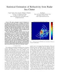
3. (INVITED) C. Yardim, P. Gerstoft, W. S. Hodgkiss, and Ted Rogers, Statistical
estimation of refractivity from radar sea clutter, IEEE Radar Conference,
Waltham, MA, April 2007.
4. C. Yardim, P. Gerstoft, and W. S. Hodgkiss, Atmospheric refractivity tracking
from radar clutter using Kalman and particle filters, IEEE Radar Conference,
Waltham, MA, April 2007.
5. C. Yardim, P. Gerstoft, and W. S. Hodgkiss, Error variance estimation in
Bayesian refractivity from clutter inversion, USNC/URSI Conference, Boulder,
CO, January 2006.
6. (INVITED) C. Yardim, P. Gerstoft, and W. S. Hodgkiss, A fast hybrid genetic
algorithm-Gibbs sampler approach to estimate geoacoustic parameter
uncertainties, Underwater Acoustic Measurements Conference, Crete, Greece,
June 2005.
7. C. Yardim, P. Gerstoft, W. S. Hodgkiss, and C.-F. Huang, Refractivity from
clutter (RFC) estimation using a hybrid genetic algorithm - Markov chain
Monte Carlo method, IEEE Antennas and Propagation & USNC/URSI Conference,
Washington DC, July 2005.
8. C. Yardim, P. Gerstoft, and W. S. Hodgkiss, Estimation of radio refractivity
from clutter using Bayesian Monte Carlo analysis, USNC/URSI Conference,
Boulder, CO, January 2005.
9. C. Yardim, P. Gerstoft, and W. S. Hodgkiss, Uncertainty analysis in the
refractivity from clutter (RFC) problem, IEEE Antennas and Propagation &
USNC/URSI Conference, Monterey, CA, June 2004.
10. A. Hizal, C. Yardim, and E. Halavut, Wideband tapered rolling strip antenna,
IEEE AP2000 Millennium Conference on Antennas & Propagation, Davos,
Switzerland, April, 2000.
11. A. Hizal, E. Halavut, C. Yardim, and A. Celebi, A linear patch antenna
array for adaptive beamforming with a spherical wave incidence, COST 260
Workshop on Smart Antennas, Aveiro, Portugal, November 1999.
Other
1. C. Yardim and P. Gerstoft, Applicability of refractivity from clutter (RFC)
method in various seas for existing radar systems, Joint MPL/UCSD – Lockheed
Martin (LM) Project Report, December, 2005.
2. C. Yardim, Design and construction of annular sector radiating line (ANSER-
LIN), microstrip helix radiating line (MISHERLIN), and tapered rolling strip
(TAROS) antennas, M.S. Thesis, 2001.
xvi

Major Field: Electrical Engineering
FIELDS OF STUDY
Studies in digital signal processing, optimization, estimation theory, detection
theory, array processing, and their applications in the atmospheric refractivity
estimation problem.
Professors William S. Hodgkiss and Kenneth Kreutz-Delgado, Dr. Peter
Gerstoft
Studies in applied ocean science, electromagnetic ducts, effects of ducting
on naval radar systems, acoustic and electromagnetic propagation in inhomogeneous
media, and their applications in radar clutter prediction for nonstandard
lower atmospheric maritime environments.
Professor William A. Kuperman, Dr. Peter Gerstoft
xvii

ABSTRACT OF THE DISSERTATION
Statistical Estimation and Tracking of Refractivity from Radar Clutter
by
Caglar Yardim
Doctor of Philosophy in Electrical Engineering
(Applied Ocean Sciences)
University of California, San Diego, 2007
William S. Hodgkiss, Chair
Kenneth Kreutz-Delgado, Co-Chair
In many maritime regions of the world, such as the Mediterranean, Persian
Gulf, East China Sea, and the Californian Coast, atmospheric ducts are common
occurrences. They result in various anomalies such as significant variations
in the maximum operational radar range, creation of regions where the radar is
practically blind (radar holes) and increased sea clutter. Therefore, it is important
to predict the real-time 3-D environment in which the radar is operating so that
the radar operator will at least know the true system limitations and in some cases
even compensate for them.
This dissertation addresses the estimation and tracking of the lower atmospheric
radio refractivity under non-standard propagation conditions frequently
encountered in low altitude maritime radar applications. This is done by statistically
estimating the duct strength (range and height-dependent atmospheric index
of refraction) from the sea-surface reflected radar clutter. Therefore, such methods
are called Refractivity From Clutter (RFC) techniques. These environmental
statistics can then be used to predict the radar performance. The electromagnetic
propagation in these complex environments is simulated using a split-step
fast Fourier transform (FFT) based parabolic equation (PE) approximation to the
wave equation.
xviii

The first part of this thesis discusses various algorithms such as genetic
algorithms (GA), Markov chain Monte Carlo samplers (MCMC) and the hybrid
GA-MCMC samplers that are used to estimate atmospheric radio refractivity for a
given azimuth direction and time. The results show that radar clutter can be a rich
source of information about the environment and the techniques mentioned above
are used successfully as near real-time estimators for the data collected during the
Wallops’98 experiment conducted by the Naval Surface Warfare Center.
The second part of this dissertation focuses on both spatial and temporal
tracking of the 3-D environment. Techniques such as the extended (EKF) and
unscented (UKF) Kalman filters, and particle filters (PF) are used for tracking the
spatial and temporal evolution of the lower atmosphere. Even though the tracking
performance of the Kalman filters was limited for certain duct types such as the
surface-based ducts due to the high non-linearity of the split-step FFT PE, they
performed well for other environments such as evaporation ducts. On the other
hand, particle filters proved to be very promising in tracking a wide variety of
scenarios including even abruptly changing environments.
xix

1
Introduction
1.1 Background
The main objective of this dissertation is to predict and improve maritime
radar performance by statistically estimating and tracking the three dimensional
real-time properties of the lower atmosphere in which the radar is operating. This
means that one has to predict the electromagnetic lower atmospheric ducts that
frequently form in many ocean and coastal regions of the world. Therefore, this
necessitates the understanding of these atmospheric events, the ability to predict
their effects on a radar system, the estimation of the environment using the
measured clutter, and finally compensating and taking necessary precautions to
counter the effects.
Hence, the work done in this dissertation involves three different fields:
1. Meteorology, for understanding the common lower atmospheric phenomena
that affect electromagnetic propagation, radar, and communication systems
operating in various environments, the atmospheric dynamics that result
in the formation of electromagnetic ducts, types of ducts and their differences,
the regions there they commonly occur, their occurrence rates, spatial
and temporal variabilities, differences between coastal and open water environments,
and the ability to forecast duct properties using meteorological
1

2
models.
2. Electromagnetic Theory, particularly radar theory and electromagnetic propagation
in inhomogeneous media, for understanding how the radar signal
propagates in complex environments, the effects of the atmospheric duct as
a leaky waveguide, interaction and scattering of the electromagnetic signal
with the sea surface for very low angle of incidence and different sea states,
incidence angle and sea clutter calculations using ray-tracing and the splitstep
fast Fourier transform based parabolic equation approximation to the
wave equation.
3. Signal Processing, for understanding how to formulate the problem in a
Bayesian framework, the statistical estimation of the environmental duct
parameters from the measured radar clutter using techniques such as genetic
algorithms (GA), different Markov chain Monte Carlo samplers (MCMC),
and hybrid GA-MCMC samplers that use nearest neighborhood and Voronoi
decomposition techniques, spatial and temporal tracking of the range, height,
azimuth and time dependent atmospheric index of refraction using various
Kalman and particle filters.
1.2 Properties of the Lower Atmosphere
The term refraction refers to the property of a medium to bend an electromagnetic
wave as it passes through the medium. The index of refraction of a
medium, n is defined as the ratio of the speed of light in vacuum to that of the
medium n = c/v. For many atmospheric applications it is simply taken as unity
since the atmospheric n changes only slightly, between 1.000250 and 1.000400 in
the lower atmosphere [1,2]. These fluctuations in the index of refraction are caused
by local changes in the temperature, pressure, and the humidity of the atmosphere.
Since the deviations are small, a new parameter N called the refractivity is defined
as the part-per-million (ppm) change in n, and is used for convenience in prop-

3
agation calculations. Due to the curvature of the Earth, an initially horizontally
propagating signal will be moving away from the surface. To take this effect into
account, the modified refractivity (M) has been introduced. N and M can be
computed as
N = (n − 1) × 10 6 = 77.6p
T
rh6.105 expx
e s =
100
x = 25.22 T − 273.2
T
+ e s3.73 × 10 5
T 2 (1.1)
( ) T
− 5.31 log e
273.2
(1.2)
(1.3)
M = N + h a × 106 (1.4)
M ≃ N + 0.157h, (1.5)
where e s is the partial pressure of water vapor, p is the barometric pressure in
millibars, T is the temperature in o K, rh is the percent relative humidity, h is the
height above the earth’s surface, and a is the radius of the Earth.
Classification of Atmospheric Conditions
Even though the fluctuations are on the order of part-per-millions, they
are sufficient to cause major changes in the tropospheric electromagnetic propagation.
Normally, the refractivity is a near-exponential function of the altitude. This
exponential can be linearized within the first kilometer or so of the atmosphere.
The slope of this linear function is –0.039 N-units/m or 0.118 M-units/m and it
usually is referred to as the “standard atmosphere”. Standard atmosphere will
result in a downward bending of the electromagnetic wave. However, this is less
than the curvature of the earth, effectively resulting in a wave that slowly moves
away from the surface. This type of propagation is called the normal propagation
condition and it occurs as long as N is between –0.079 to 0 N-units/m (0.079 to
0.157 M-units/m).
If N has a positive slope with respect to the altitude, the wave will further
bend upward creating the sub-refractive conditions, which only infrequently occurs

4
in nature.
On the other hand if the N-gradient continues to decrease it can reach
a critical value of –0.157 N-units/m (0 M-units/m). At this point the downward
bending caused by refraction exactly matches the curvature of the earth creating
an electromagnetic wave propagating horizontally to the surface. The condition
where the refraction strength is between the normal and this critical value is called
the super-refraction condition.
Figure 1.1: Tropospheric propagation conditions. Sub-refraction, standard refraction,
super-refraction, and trapping (ducting). (Figure taken from [1])
If the negative N-gradient is even stronger than the critical value, the wave
will be forced to bend downward, eventually hitting the surface. However, since the
surface-reflected wave will reenter the strongly negative N-gradient region it will
again be bent down bouncing multiple times from the surface as shown in Fig. 1.1.
It effectively will be trapped between the surface and an imaginary upper boundary
creating a waveguide with an open leaky top wall called an electromagnetic duct.
Therefore this condition is called the trapping condition. These conditions are
summarized in Table 1.1.

5
Table 1.1: Tropospheric Propagation Conditions
∂N
Atmospheric Condition (N-units/m) ∂M
(M-units/m)
∂z ∂z
Standard –0.039 0.118
Sub-refraction >0 >0.157
Normal –0.079 - 0 0.079 - 0.157
Super-refraction –0.157 - –0.079 0 - 0.079
Trapping

6
over the coastal regions and the ocean) very strong sea ducts of several hundred
kilometer size can be formed, lasting for days. Typical examples that induce strong
duct formations include the Santa Ana of southern California, the Sirocco of the
southern Mediterranean, and the Shamal of the Persian Gulf.
The sea duct essentially is a fine-weather phenomenon. Since it requires
a strongly stratified atmosphere for temperature and humidity inversion, a well
mixed atmosphere due to poor weather conditions will prevent sea duct formation.
Rough terrain, high winds, cold, stormy, rainy, and cloudy conditions usually will
result in more uniform vertical temperature and humidity profiles, decreasing duct
formation. Therefore ducting is more common in equatorial, tropical, and subtropical
regions. Ducting is further enhanced in these regions due to the high
evaporation rate. The same is true for the summer and day time ducts [1,2].
(a)
Evaporation
Duct
(b)
Surface
Based
Duct
(c)
Elevated
Duct
Height
Evaporation
Duct Height
Height
Trapping
Layer
Height
Trapping
Layer
Modified Refractivity M
Modified Refractivity M
Modified Refractivity M
Figure 1.2: Most common three duct types. Evaporation, surface-based, and elevated
ducts.
There are three major sea ducts frequently encountered in the lower atmosphere
(Fig. 1.2):
1. Evaporation ducts (ED) are formed due to the inherent humidity inversion
at the air/sea boundary. They are the most commonly encountered type of
sea ducts. The air in contact with the sea is saturated with water vapor
and the water vapor decreases approximately as a logarithmic function of
height creating the evaporation duct structure given in Fig. 1.2 (a). The

7
height at which the modified refractivity M becomes minimum is called the
evaporation duct height (EDH). ED formation is a strong function of latitude
since the necessary evaporation rates required cannot be sustained in colder
regions. For example, an evaporation duct with an EDH> 10 m occurs 92 %
of the time in the coastal regions of northern Brazil, whereas this number is
only 2 % at Bering Strait. EDH will very rarely be more than 40 m and the
world average is 13 m.
2. Surface-based ducts (SBD) are formed when sharp humidity and temperature
inversions occur due to the advection of warm and dry air over the ocean.
The humidity gradient is usually further enhanced due to the evaporation
from the sea surface. They are less common than the evaporation ducts
but usually have a more pronounced effect on electromagnetic propagation.
They typically are represented by a tri-linear profile with a negatively-sloped
trapping layer as given in Fig. 1.2 (b). When the bottom of the trapping layer
touches the sea surface, the SBD is sometimes referred to as a surface duct.
In both the SBD and ED, the sea surface serves as the bottom boundary for
the leaky electromagnetic waveguide.
3. Elevated ducts (ElevD) are formed due to the presence of marine boundary
layers. The resultant inversion is called tradewind inversion, generating an
strong duct at the top of the marine boundary layer. Elevated duct also has
a tri-linear profile similar to a SBD as given in Fig. 1.2 (c). Elevated ducts
are formed essentially from the same meteorological conditions as a SBD. In
fact, coastal SBD’s can slope upward to become elevated ducts. Similarly,
a tradewind inversion may intensify, turning an elevated duct into a SBD.
Elevated ducts usually occur at altitudes much higher than the SBD. For
example the average elevated duct height is 600 m and 1500 m, respectively
for the southern California coast and the coast of Japan. The fundamental
difference between an elevated duct and other duct types is that the duct

8
is no more bounded below by the sea surface. This is especially important
for RFC, since the ducting conditions are inferred from the surface-reflected
sea clutter. Since elevated ducts do not interact with the surface, the RFC
techniques discussed in this dissertation cannot be used for elevated duct
prediction.
Annual regional statistics of different regions throughout the world are
given in Table 1.2.
Table 1.2: Some Regional Duct Statistics
Percent Occurrence (Annual Averages)
Region ED>10 m SBD ElevD multi–Elev. Elev.+SBD
D N D N D N D/N Avg. D/N Avg.
Persian Gulf 77 62 36 52 26 33 2.8 4.8
Gulf of Mexico 84 79 9 10 38 40 8.3 2.6
East China Sea 83 76 10 7 15 18 3.4 2.0
(Indian Ocean)
Diego Garcia 87 76 34 18 20 37 7.3 3.8
(Atlantic Ocean)
Rio Grande do Nor. 92 87 18 18 24 30 6.8 7.2
East Mediterranean 72 62 13 11 12 16 2.4 2.5
West Mediterranean 58 45 15 14 10 12 1.7 2.6
Yellow Sea 63 56 16 13 17 18 7.0 3.4
Southern California 46 35 23 15 33 38 5.6 3.2
Baltic Sea 12 8 2 3 3 4 0.6 0.4
Bering Strait 2 1 6 5 4 5 1.1 0.8
1.2.2 Effects of Ducts on Naval Radar and Communication Systems
Even though the sub-refractive and super-refractive conditions are important
in their own right, they do not result in a major change in the shape of the
coverage diagram of a radar. On the contrary, trapping conditions will fundamen-

9
tally alter the propagation characteristics, the coverage area, and hence almost all
of the important radar parameters as shown in Fig. 1.3.
The M-profile structure seen in Fig. 1.3 (a) is a weak evaporation duct.
Notice how the value of M increases at a rate of 0.118 M-units/m except for the
evaporative region near the surface. Since the evaporation duct is very weak it
does not affect the propagation as seen from its coverage diagram obtained using
the split-step fast Fourier transform (FFT) parabolic equation (PE). The upward
bending effect of the normal propagation conditions can be seen clearly. Since the
signal is bend upward, it has minimal interaction with the sea surface resulting
in a clear clutter map, defined as the clutter observed on the radar plan position
indicator (PPI).
150
(a)
-110
150
(b)
-110
100
-130
100
-130
50
50
-150
300 350 20 60 100 140
Refractivity (M-unit/m) Range (km)
Reflectivity image: March 11, 1998 Map # 031198-20 15:52:33.3
-250
-150
300 350 20 60 100 140
Refractivity (M-unit/m) Range (km)
Reflectivity image: April 02, 1998 Map # 040298-17 18:50:00.3
40 -250
40
-200
35 -200
35
-150
-100
-50
-150
30
-100
25
-50
30
25
0
50
100
150
50 km
100 km
150 km
200 km
20 0
50
15
100
10
150
50 km
100 km
150 km
200 km
20
15
10
200
5
200
5
250
-200 -100 0 100 200
0
250
-200 -100 0 100 200
0
Figure 1.3: Vertical M-profiles, coverage diagrams, and clutter maps resulting from
(a) a weak evaporation duct and (b) a strong surface-based duct.

10
Fig. 1.3 (b) shows what happens in the event of the formation a lower
atmospheric duct. The coverage diagram is now entirely changed with a complex
waveguide-like propagation pattern within the duct. Since the electromagnetic
wave is trapped, it interacts heavily with the surface, resulting in an increase in
the sea clutter observed by the radar. With each bounce, a small portion of the
signal is scattered depending on the surface roughness and observed by the radar
as shown on the radar PPI. Since the surface bounces occur at certain ranges as
shown in the coverage diagram, it results in the formation of clutter rings around
the radar on the PPI screen. The RFC techniques introduced in this dissertation
uses this effect to estimate and track the atmospheric ducting conditions.
Figure 1.4: Effects of ducting on naval and communication systems.(Figure taken
from [1])
The propagation changes discussed above result in important deviations
in the radar/communication system characteristics as shown in Fig. 1.4. An important
effect of ducting is the change in the maximum radar detection/communication
channel range. For example, the range can be reduced significantly outside the duct
since most of the electromagnetic signal is trapped within the duct. These areas
are called radar holes. On the contrary, the maximum detection range within the

11
duct increases typically from two to five times that of a standard atmospheric
case [2].
Moreover, ducting will also cause altitude errors in the target location
due to the strong bending of the wave. System performance may also suffer from
increased sea clutter.
1.2.3 Measurement of Duct Properties
The most accurate way of measuring the atmospheric refractivity profile is
using a microwave refractometer [2,3]. It measures the index of refraction directly
by using cavity resonance. It is composed of two microwave cavities fed by the
same source. One is an open cavity that will collect the sample of atmosphere
and the other one is a sealed cavity acting as a reference. The difference in the
resonance frequencies will indicate how much difference there is between the two
media, enabling the measurement of the n of the environment. Even with its very
high accuracy and measurement speed refractometers are expensive and must be
used with a helicopter or plane flying in a sawtooth pattern to obtain the two
dimensional height and range dependent profile greatly limiting their usage.
The most common measurement technique is measuring n indirectly from
the atmospheric temperature, humidity and pressure profiles, and using these in
(1.1). Radiosonde balloons [4] that carry conventional weather observation instruments
to measure these three environmental parameters are used for this purpose.
Their shortcomings are the slow response time (typically 30 min. to get a vertical
profile), slow update rate (typically one launch every two to twelve hours),
inability to obtain range-dependent profiles, local heat sources lowering the accuracy
(especially the effect of the metallic body of the ship it is launched from),
non-vertical sampling due to the horizontal drift resulting from the wind, the need
of extra hardware and measurement, and the associated cost for these hardware.
These drawbacks also are valid for the rocketsondes that essentially do the same
thing.

12
Doppler spread radars [5] are another way of gathering information about
the environment. Although they do not directly measure the refractivity profile,
they provide detailed temporal and spatial pictures of the structure parameter Cn
2
describing the turbulent perturbations in the refractivity. This theoretically can be
used to extract refractivity itself. However, in practice, clouds, other contaminants,
the need for a high signal to noise ratio, and contamination of the doppler spectrum
due to non-turbulence related processes limit the effectiveness of the technique.
One other option is to forecast the ducting conditions using atmospheric
prediction models. One such has recently been developed by the US Navy. The
Coupled Ocean/Atmosphere Mesoscale Prediction System (COAMPS), developed
by the Naval Research Laboratory (NRL), is a high-resolution, local weatherprediction
model coupled with a powerful data assimilation code that integrates regional
and satellite measurements [6,7]. It can provide a range-dependent “ducting
forecast” anywhere around the world and usually updates every 12 hours. However,
COAMPS also has limited capabilities and the M-profile predictions near the
surface have relatively poor accuracy.
Another technique that can infer the refractivity is the lidar [8] techniques
such as the differential absorption lidar (DIAL) and the Raman lidar. Lidars
are used to measure the temperature and water vapor profiles. DIAL uses
the strong wavelength-dependent absorption characteristics of atmospheric gases.
Raman-scattering lidars utilize a weak molecular scattering process which shifts
the incident wavelength by a fixed amount associated with rotational or vibrational
transitions of the scattering molecule. They can measure both horizontal
and vertical variations and are much faster than radiosondes. Disadvantages of
lidar are that it is a more complex technique using expensive equipment and that
lidars are limited by daytime background radiation and aerosol extinction.
The Global Positioning System (GPS) technique [9] is an attempt to
use GPS satellites to infer the atmospheric environment. Similar to the radar
signal, a GPS signal from a rising or setting satellite just over the horizon will

13
be distorted while propagating through the duct. Therefore, it may be possible
to get information about the environment through which the GPS signal passes.
This method estimates duct parameters by matching the delays in the received
GPS signal using a ray-tracing code. Although still under development, GPS
measurements may be a promising alternative to the radiosonde measurements
due to higher update rates.
Finally, one can use the radar itself to gather information about the environment.
The prospect of using the radar itself during its normal operation
without needing any other hardware or extra measurements makes the refractivity
from clutter (RFC) technique a promising alternative and addition to the methods
provided above. It would only require the radar clutter, the normally filtered-out
and discarded part of the radar signal, as its input. The technique potentially can
provide the estimation and tracking of the range, azimuth and time-dependent
three-dimensional cylindrical refractivity profile with the radar at its center. However
it should also be noted that, similar to the techniques above, RFC comes
with its own limitations and assumptions as discussed in detail throughout the
dissertation.
1.3 Electromagnetic Propagation in the Lower Atmosphere
The electromagnetic theory section can be split into two sections. First
one describes the split-step fast Fourier transform parabolic equation approximation
to the wave equation used in this work and the other describes the extraction
of the radar clutter return in this complex environment using the radar equation,
taking into account the very low-angle sea surface radar cross section and the
adjustment in the propagation loss due to the non-standard propagation.

14
1.3.1 Tropospheric Propagation Using Split-Step Fast Fourier Transform
Parabolic Equation
Computation of the electromagnetic propagation in the atmosphere usually
means solving the Maxwell’s equations for a very large domain of interest with
respect to the wavelength. This makes it impossible to solve the exact problem and
approximations are made to simplify the problem to a manageable size. For many
years, approximate methods such as the geometrical optics and mode theory have
been used in tropospheric propagation calculations involving complex refraction
problems such as the non-standard propagation formed under ducting conditions.
These methods were largely replaced in 1990’s by the parabolic equation (PE) following
the introduction of the method in [10]. The formulation developed below
is based on the ones given in [11–14]. Two different PE codes are used throughout
this dissertation; our own code developed following [14] that is embedded into
our Monte Carlo sampler and tracking algorithm codes, and the Terrain Parabolic
Equation Model (TPEM) code written by Amalia E. Barrios [13].
Assuming a time harmonic variation of e −jwt , the two dimensional cylindrical
scalar wave equation for the electromagnetic field ψ(r, z) in a homogeneous
medium with a refractive index n can be written as
∂ 2 ψ
∂r + 1 ∂ψ
2 r ∂r + ∂2 ψ
∂z + 2 k2 n 2 ψ = 0, (1.6)
where k is the wave number, r and z are range and height of the cylindrical coordinates
(r, θ, z), respectively. However, in reality the index of refraction will not be
constant in our inhomogeneous medium but a function of r and z as n(r, z). But
since the variation in n will almost always be very small relative to the wavelength,
(1.6) is still a highly accurate approximation.
An electromagnetic field trapped within the duct would have a canonical
outgoing solution to the wave equation in cylindrical coordinates in terms of a
Hankel function H0 1 (kr) of the first kind and of order 0. Since the Hankel function
can be represented by the first order term in its asymptotic expansion in the

15
far-field, one can define the reduced function u(r, z) in terms of the field ψ(r, z)
propagating in the r-direction as
H 1 0 (kr) ≃ √
2
πkr ej(kr− π 4 ) (1.7)
u(r, z) = √ kre −jkr ψ(r, z). (1.8)
where the square root term represents the decay in cylindrical spreading (1/ √ r
compared to the 1/r decay term of the classical spherical spreading). Inserting
(1.8) into (1.6) one can obtain the wave equation for a flat earth given by
{ ∂
2
∂r + 2jk ∂ }
2 ∂r + ∂2
∂z + 2 k2 (n 2 − 1) u(r, z) = 0, (1.9)
which can be factored as
{ ∂
∂r + jk(1 − Q) }{ ∂
∂r + jk(1 + Q) }
u(r, z) = 0. (1.10)
Q in (1.10) is a pseudo-differential operator defined by
Q (Q(u)) = 1 k 2 ∂ 2 u
∂z 2 + n2 u. (1.11)
By defining a special square root function that corresponds to the composition of
operators one can formally define Q as
√
1 ∂
Q =
2
k 2 ∂z + 2 n2 (r, z). (1.12)
Finally one can define a function Z such that
Z = 1 k 2 ∂ 2
∂z 2 + (n2 − 1) (1.13)
Q = √ 1 + Z. (1.14)
One should note that there are inherent errors in the factorization given in (1.10).
If the index of refraction n varies considerably with range, then the operator Q
does not commute with the range derivative and the factorization fails.

16
Now the wave equation can readily be split into outgoing and incoming
field components, each corresponding to a parabolic equation
∂u +
∂r = −jk(1 − Q)u + (1.15)
∂u −
∂r = −jk(1 + Q)u −, (1.16)
where u + and u − correspond to the forward and backward propagating waves, respectively.
Assuming that the backward propagating part of the wave is negligible
so that all the energy propagates in the forward direction the wave equation will
have a solution given by
u(r + △r, z) = e jk△r(−1+Q) u(r, z). (1.17)
This equation can be solved by marching techniques given the initial vertical field
profile at a desired initial range, and the necessary boundary conditions on the
bottom and top of the domain. The bottom of the domain is the sea/air interface
usually taken as a perfect electric conductor (PEC) boundary layer. The top is
an open infinite boundary condition so the artificially created domain truncation
will require an absorbing boundary condition to prevent the signal going upwards
from reflecting back into the region of interest.
The simplest approximation of (1.15) is obtained by using the first order
Taylor series expansions of the square root and exponential functions.
Q = √ 1 + Z ≃ 1 + Z 2
(1.18)
This yields the standard parabolic equation (SPE)
∂ 2 u(r, z) ∂u(r, z)
+ 2jk + k 2 (n 2 (r, z) − 1)u(r, z) = 0. (1.19)
∂z 2 ∂r
Note that (1.19) is exactly the same as the original equation (1.9) with the first term
dropped. This is because all the intermediate steps and approximations covered
above can be combined into a single narrow-angle condition called the paraxial or
parabolic approximation where
∣ ∣ 2k
∂u
∣∣∣ ∣∂r
∣ ≫ ∂ 2 u ∣∣∣
, (1.20)
∂r 2

17
which results in the cancelation of the first term in (1.9). Therefore, to approximate
the wave equation in this parabolic equation form the following conditions must
be satisfied [14]:
1. The equation is only valid within a narrow beam geometry called the paraxial
cone, typically not more than 10 o . The first order error term associated with
increased propagation angle is proportional to sin 4 α, where α is the angle
between the propagation direction and the horizontal paraxial direction r.
This error term will increase with α as 10 −7 , 10 −3 , and over 10 −2 for 1 o , 10 o ,
and 20 o , respectively. More computationally expensive wider angle schemes
can be implemented using the Padé coefficients however lower atmospheric
duct calculations will typically require an angle less than 0.5 o (see Fig. 1.5)
making the fast narrow angle code preferable to wide angle finite difference
schemes.
2. The field is valid only in the far-field, not close to the source.
3. The medium is only weakly inhomogeneous such as the part-per-million
changes involved here.
4. Most of the energy should be propagating forward without any significant
back scattering.
Equation (1.17) can be marched using the split-step fast Fourier transform
(FFT) method, where u(r, z) and U(r, p) are Fourier transform pair related by
∫ zmax
U(r, p) = F {u(r, z)} = u(r, z)e −jpz dz (1.21)
−z max
u(r, z) = F −1 {U(r, p)} = 1 ∫ pmax
u(r, z)e jpz dp, (1.22)
2π −p max
where the transform variable is defined by p = k sin α, and the domain truncation
height is related to p max using the Nyquist criteria z max p max = Nπ, N being the
FFT size. Taking the FFT of the SPE (1.19) one can compute the closed form

18
solution for U(r, p) as
−p 2 ∂U(r, p)
U(r, p) − 2jk + k 2 (n 2 − 1)U(r, p) = 0 (1.23)
∂r
U(r, p) = e −jp2 r/(2k) .e jk(n2 −1)r/2 , (1.24)
which will result in a marching solution of
}
u(r + △r, z) = e jk(n2−1)△r/2 F
{e −1 −jp2△r/(2k) F {u(r, z)} . (1.25)
An important step is the inclusion of the correction term in the first exponential
due to the earth flattening transformation. This will replace n 2 with the modified
index of refraction m 2 where
m(r, z) = n(r, z)e (z/a) ≃ n + z , 0 ≤ n − 1 ≪ 1, z ≪ a (1.26)
[
a
M(r, z) = n(r, z) − 1 + z ]
× 10 6 (1.27)
a
m 2 − 1 ≃ 2(m − 1) = 2M(r, z) × 10 −6 . (1.28)
Although not critical for our case, a final improvement in (1.25) is obtained by
using a slightly improved wide angle approximation given in [13]. This will finally
result in the split-step FFT parabolic equation used throughout this dissertation
with a marching step given by
]
u(r + △r, z) = exp
[ik o △rM(r, z)10 −6 × (1.29)
[ (√ )] }
F
{exp
−1 i△r k2 − p 2 − k F {u(z, r)} .
A normalized Gaussian antenna pattern is used here as the starter field with
U(r o , p) = e −p2 w 2 /4
(1.30)
√
2 ln2
w =
k sin ( )
α BW
(1.31)
2
where α BW is the half power beamwidth. A launch angle other than the horizontal
is achieved by simply replacing U(r o , p) with U(r o , p − p o ), with p o = ksinα o .
It should be noted that at high altitudes the earth flattening transformation
given here becomes less accurate. Moreover, the modified index of refraction

19
becomes large at high altitudes making the narrow-angle scheme inaccurate at
more than a few kilometers. However, the form given in (1.29) totally satisfies all
accuracy needs of the lower atmospheric narrow-angle ducted propagation environments
simulated in this work.
1.3.2 Radar Sea Clutter Calculation Under Non-Standard Propagation
Conditions
Using the classical radar equation, received radar clutter power can be
written as
P c
= P tG 2 t λ2 F 4 σ
(4π) 3 R 4 , (1.32)
where P t is the transmitter power, G t is the transmit antenna gain, λ is the wavelength,
σ is the sea surface radar cross section (RCS), R is the range, and F is the
propagation factor (ratio of the electric field at a point to that which would have
been created by the same system operating in free space with the on-axis gain of
the antenna) [15]. After F is calculated at the effective scattering height given as
0.6 times the mean wave height [16], the one-way propagation loss L then can be
written as
L fs
L = L fs /F 2 (1.33)
= (4πR)2
λ 2 , (1.34)
where L fs is the free space loss. Sea surface RCS can be written as σ = A c σ o ,
where A c is the illuminated area (proportional to R at small grazing angles) and
σ o is the normalized sea surface radar cross section (RCS). Then the clutter power
can be written as
P c
= P tG 2 t 4πA cσ o
L 2 λ 2 (1.35)
P c = Cσo R
L 2 (1.36)
P c,dB = −2L dB + σ o (R) dB + 10 log 10 (R) + C dB , (1.37)

20
where C accounts for all the constant terms [17].
In reality, both σ o and F are functions of grazing angle, the effective
clutter height (which itself is a function of average wave height at the sea), range
and duct parameters. Hence, they can only be accurately calculated after the
forward model run with the additional knowledge of wind speed and direction.
There are various models such as the Georgia Institute of Technology model (GIT)
and hybrid model (HYB) and in present codes such as the Advanced Refractive
Effects Prediction System (AREPS), a modified GIT is used [1,16,18].
The grazing angle Ψ o dependence for vertical polarization is still an active
research subject. It is not easy to determine the exact nature of the dependence
of the sea surface RCS to the grazing angle and dependencies between Ψ 0 o and Ψ 4 o
are reported in the literature [19,20]. However, one main problem is that many of
these studies are done under conditions where either there is no ducting or where
there is no information about the duct. In his evaporation duct height inversion
paper [21], Rogers et al. report that while the data did not provide a definitive
answer to the grazing angle dependency problem, the use of σ o ∝ Ψ 0 o generated
the best results in his duct height estimation algorithm.
One interesting difference of a ducted environment relative to the standard
atmospheric conditions is that, as the electromagnetic wave gets trapped and
propagates inside the duct, the surface grazing angle converges to a constant value.
This phenomenon is very unlike the 1/R variation of Ψ o with respect to the range
that would be observed in a low-angle non-ducting atmosphere. Hence, regardless
of the assumed dependence of the sea surface RCS on the grazing angle, the grazing
angle and hence σ o will become constant under ducting conditions after a certain
range value. This assumes similar conditions such as the wind profile throughout
the desired range interval. To show this, an electromagnetic ray-tracing is performed
to observe the dependence of Ψ o on the ducting conditions as a function of
range as given in Fig. 1.5. It can clearly be seen that for long ranges the grazing
angle is almost constant and the minimum range where one can assume a constant

21
Ψ o decreases as the strength of the duct increases.
Combining this fact with the observations given in [21] (that σ o ∝ Ψ 0 o , i.e.
independent, or at most weakly dependent), one could arguably state that rangedependence
of σ o in (1.37) can be dropped if only the power clutter at ranges larger
than a R min is used in the inversion. This value is selected to be 12 km in [21] and
a value of 10 km has been used throughout this dissertation.
One other practical problem is the level of the clutter signal at longer
ranges. The Space Range Radar (SPANDAR) used to measure the radar clutter in
the Wallops Island experiments used in this thesis is a high power, high gain system
relative to a sea-borne naval radar. It can achieve typically a 40 dB clutter-to-noise
ratio (CNR) at 10 km range with CNR dropping to 0 dB anywhere between 30 to
50 km for an evaporation duct environment depending on various other conditions
such as the wind and ducting strength. An average naval system will probably
have a 0 dB CNR at 20-25 km. This value is typically much higher in surfacebased
duct cases. This limits the maximum range of the clutter that can be used in
the inversion. R max values of 25 km and 60 km (the main reason for the selection
of 60 km in the SBD case is because the helicopter measurements are limited to
0-60 km range, not the lack of clutter power) are selected for the evaporation and
surface-based ducts, respectively, throughout this dissertation.
To summarize, the main issue here in a practical system will be the selection
of ranges which will be used in the inversion. Short ranges are preferred
since at close ranges the returned clutter is larger (high CNR), whereas constant
grazing angle assumption is more accurate at longer ranges. The selected values
will also strongly depend on the radar parameters, especially its height, power and
gain and the mean environment the radar will be operating in. Depending on
the system, GIT or modified GIT clutter models may be more accurate than the
assumptions used in this work. Ranges between 10-25 km and 10-60 km are used
in this dissertation for the evaporation duct inversions and the surface-based duct
inversions, respectively.

22
Figure 1.5: Sea surface grazing angle as a function of range for different evaporation
duct heights computed using ray-tracing.
1.4 Statistical Estimation and Tracking
A Bayesian framework was adopted throughout this dissertation. All the
environmental parameters were selected as random variables with posterior probability
density functions (pdf’s). This statistical estimation allowed the projection
of the environmental probabilities into the pdf’s of parameters-of-interest as shown
in Fig. 1.6. Measured data d, which is the radar clutter return, is mapped into a
posterior distribution p(m|d) of environmental duct parameters m. The environmental
parameters are then mapped into the usage domain U as p(u|d) via Monte
Carlo integration. u typically constitutes the propagation factor (F) or the oneway
transmission loss (L) so that p(u|d) can be used in radar calculations such as
the detection probability (P D ), two-dimensional coverage diagrams and the false

23
alarm rate.
Environmental
domain
Data domain
d
m
Usage domain
Utility u
Figure 1.6: An observation d is mapped into a distribution of environmental parameters
m that potentially could have generated it. These environmental parameters
are then mapped into the usage domain u.
The list of techniques used in this work are given as below. Each of these
techniques is summarized in their prospective chapters.
• Genetic Algorithms (GA)
• Simulated Annealing (SA)
• Metropolis-Hastings (MCMC) Sampler
• Gibbs (MCMC) Sampler
• Hybrid GA-MCMC Sampler
• Extended Kalman Filter (EKF)
• Unscented Kalman Filter (UKF)
• Sequential Importance Resampling Particle Filter (SIR-PF)
1.5 Scope of This Dissertation
The major contents of this dissertation consist of three chapters, Chapters
2 to 5 1 . The first two of these chapters deals with the statistical estimation of the
1 Each chapter is essentially a full or partial reprint of papers that are published, accepted, or submitted
to a professional journal. Therefore, each has been written in a paper format and is self-contained.

24
atmospheric index of refraction while Chapter 5 covers the spatial and temporal
tracking of it.
Chapter 2 is devoted to the analysis of the RFC inversion problem using
different Markov chain Monte Carlo samplers (MCMC) [22]. A typical rangeindependent
tri-linear surface-based electromagnetic duct is estimated statistically
using Metropolis-Hastings [23] and Gibbs [24] samplers. The main purpose is estimating
statistically the uncertainties in the environmental parameters and projecting
these into the posterior probability densities of transmission loss and propagation
factor using Monte Carlo integration that can be used to predict and in some
cases correct the radar performance operating in such an environment. The results
are checked with exhaustive search and compared with previous studies conducted
using genetic algorithms [17]. The methods are then successfully tested on data collected
during the Wallops Island 1998 experiment conducted by the Naval Surface
Warfare Center, Dahlgren Division that included both range-dependent environmental
refractivity measurements using the helicopter provided by the Applied
Physics Laboratory, John Hopkins University and radar clutter maps obtained
during the operation of the Space Range Radar (SPANDAR). The results showed
that these methods can accurately compute the required Monte Carlo integrations
but needed high number of forward model runs which are composed of propagating
the electromagnetic signal in these complex environments using the split-step FFT
PE method and hence are not suitable for a real or near-real time statistical RFC
estimator. Moreover, inclusion of range-dependence results in an increase in the
number of environmental parameters to be estimated and an increased dimension
of the parameter state-space, making these algorithm even less suitable for realtime
applications. This resulted in a search for techniques that would necessitate
fewer forward model runs with a minimal degradation in the MCMC performance.
This problem is addressed in Chapter 3. A hybrid genetic algorithms
(GA) – Markov chain Monte Carlo method [25] based on the nearest neighborhood
algorithm proposed in [26,27] is implemented. This method uses a Voronoi

25
decomposition scheme that divides the entire state space into Voronoi cells, effectively
discretizing the entire multi-dimensional state space. These cells are centered
around the set of samples obtained from the entire set of generations of populations
of the preceding genetic algorithms run. This creates an approximation to
the environmental posterior density, which subsequently is resampled by a MCMC
sampler such as the Gibbs algorithm to accurately compute the necessary MC
integrals. This method removes computation of the forward model during the resampling
MCMC phase and can result in a large reduction in the forward model
runs required. The hybrid method is compared with the classical MCMC samplers
used in the previous chapter. The results showed that accurate MC integrals can
be computed using much smaller set of GA samples. Then the method is successfully
used to estimate an range-dependent inversion of the environment in the
Wallops Island 1998 experiment data.
Chapter 4 treats the RFC problem as a real-time tracking problem [28–
31]. The purpose is to perform a real-time tracking of the three dimensional environment
within a circular radius centered on the radar system. This requires both
temporal and spatial tracking of the environmental parameters. The problem is
non-linear due to the split-step FFT PE and usually non-Gaussian due to the prior
densities obtained from either inversions performed in Chapters 2 and 3 or from
some other source such as the regional statistics or COAMPS forecasts. Moreover,
the strength of the non-linearity depends on the environment. For example,
surface-based and mixed type ducts show highly nonlinear electromagnetic propagation
characteristics whereas evaporation ducts result in only mild non-linearities.
This necessitates implementation and comparison of different types of tracking filters
for different scenarios that are commonly encountered in maritime regions.
The advantages and drawbacks of each filter and selection of the best possible filter
for various environmental conditions are addressed. Three filters, namely the
extended Kalman (EKF), unscented Kalman (UKF), and particle filters (PF), are
used [32]. The Sequential Importance Resampling (SIR) algorithm is used in the

26
implementation of the PF. Both Kalman filters performed poorly in surface-based
duct environments with high-nonlinearities. On the contrary, the PF performed
well in these environments with a mean square error (MSE) converging to that
predicted by the posterior Cramér-Rao lower bound (PCRLB). The Kalman filters
performed much better in evaporation duct tracking applications.
Finally, Chapter 5 addresses the conclusions of this dissertation and suggestions
for possible future work.

27
Bibliography
[1] Space and Naval Warfare Systems Center, Atmospheric Propagation Branch,
San Diego, CA. User’s Manual for Advanced Refractive Effect Prediction
System, 3.4 edition, April 2005.
[2] Merrill I. Skolnik. Introduction to Radar Systems. McGraw–Hill, New York,
third edition, 2001.
[3] J. H. Richter. Sensing of radio refractivity and aerosol extinction. IEEE
Geoscience and Remote Sensing Symposium, IGARSS’94, 1:381–385, 1994.
[4] J. R. Rowland and S. M. Babin. Fine-scale measurements of microwave profiles
with helicopter and low cost rocket probes. Johns Hopkins APL Tech. Dig.,
8 (4):413–417, 1987.
[5] J. H. Richter. High resolution troposheric radar sounding. Radio Science,
4(12):1261–1268, 1969.
[6] Cory A. Springer. The gouge on COAMPS: What is it? why use it? how to
use it. Naval Meteorology & Oceanography Command News, 19(2), 1999.
[7] Naval Research Laboratory, Monterey Marine Metrology Division. Coupled
Ocean/Atmosphere Mesoscale Prediction System (COAMPS) Web Page, 3.1.1
edition, 2004.
[8] Adam Willitsford and C. R. Philbrick. Lidar description of the evaporative
duct in ocean environments. volume 5885. Proceedings of SPIE, Bellingham,
WA, September 2005.
[9] Anthony R. Lowry, Chris Rocken, Sergey V. Sokolovskiy, and Kenneth D.
Anderson. Vertical profiling of atmospheric refractivity from ground-based
GPS. Radio Science, 37(3):1041–1059, 2002. doi:10.1029/2000RS002565.
[10] H. W. Ko, J. W. Sari, and J. P. Skura. Anomalous wave propagation through
atmospheric ducts. Johns Hopkins APL Tech. Dig., 4:12–26, 1983.
[11] G. D. Dockery. Modeling electromagnetic wave propagation in the troposphere
using the parabolic equation. IEEE Trans. Antennas Propagat., 36 (10):1464–
1470, 1988.

28
[12] Amalia E. Barrios. Parabolic equation modeling in horizontally inhomogeneous
environments. IEEE Trans. Antennas Propagat., 40 (7):791–797, 1992.
[13] Amalia E. Barrios. A terrain parabolic equation model for propagation in the
troposphere. IEEE Trans. Antennas Propagat., 42 (1):90–98, 1994.
[14] M. Levy. Parabolic Equation Methods for Electromagnetic Wave Propagation.
The Institution of Electrical Engineers, London, United Kingdom, 2000.
[15] David Barton. Modern Radar System Analysis. Artech House, Norwood, MA,
1988.
[16] J. P. Reilly and G. D. Dockery. Influence of evaporation ducts on radar sea
return. IEE Proc. Radar and Signal Processing, 137 (F–2):80–88, 1990.
[17] Peter Gerstoft, L. T. Rogers, J. Krolik, and W. S. Hodgkiss. Inversion for
refractivity parameters from radar sea clutter. Radio Science, 38 (3):1–22,
2003. doi:10.1029/2002RS002640.
[18] G. D. Dockery. Method of modelling sea surface clutter in complicated propagation
environments. IEE Proceedings, 137 (F–2):73–79, 1990.
[19] D. E. Barrick. Grazing angle behavior of scatter and propagation above any
rough surface. IEEE Trans. Antennas Propagat., 46(1):73–83, 1998.
[20] V. I. Tatarski and Charnotskii M. On the behaviour of scattering from a
rough surface for small grazing angles. IEEE Trans. Antennas Propagat.,
46(1):67–72, 1998.
[21] L. Ted Rogers, C. P. Hattan, and J. K. Stapleton. Estimating evaporation
duct heights from radar sea echo. Radio Science, 35 (4):955–966, 2000.
doi:10.1029/1999RS002275.
[22] Caglar Yardim, Peter Gerstoft, and William S. Hodgkiss. Estimation of radio
refractivity from radar clutter using Bayesian Monte Carlo analysis. IEEE
Trans. Antennas Propagat., 54(4):1318–1327, 2006.
[23] N. Metropolis, A. W. Rosenbluth, M. N. Rosenbluth, A. H. Teller, and
E. Teller. Equation of state calculations by fast computing machines. J.
of Chemical Physics, 21:1087–1092, 1953.
[24] S. Geman and D. Geman. Stochastic relaxation, Gibbs distributions, and the
Bayesian restoration of images. IEEE Trans. Pattern Anal. Machine Intell.,
6:721–741, 1984.
[25] Caglar Yardim, Peter Gerstoft, and William S. Hodgkiss. Statistical maritime
radar duct estimation using a hybrid genetic algorithms – Markov chain Monte
Carlo method. Radio Science, in press.

29
[26] Malcolm Sambridge. Geophysical inversion with a neighborhood algorithm -
I. searching a parameter space. Geophys. J. Int., 138:479–494, 1999.
[27] Malcolm Sambridge. Geophysical inversion with a neighborhood algorithm -
II. appraising the ensemble. Geophys. J. Int., 138:727–746, 1999.
[28] Caglar Yardim, Peter Gerstoft, and William S. Hodgkiss. Tracking refractivity
from clutter. IEEE Trans. Antennas Propagat., submitted.
[29] Caglar Yardim, Peter Gerstoft, and William S. Hodgkiss. Atmospheric refractivity
tracking from radar clutter using Kalman and particle filters. IEEE
Radar Conference, Boston, MA, April 2007.
[30] Caglar Yardim, Peter Gerstoft, and William S. Hodgkiss. Tracking atmospheric
ducts using radar clutter: I. evaporation duct tracking using Kalman
filters. IEEE APS Conference, Honolulu, Hawaii, June 2007.
[31] Caglar Yardim, Peter Gerstoft, and William S. Hodgkiss. Tracking atmospheric
ducts using radar clutter: II. surface-based duct tracking using multiple
model particle filters. IEEE APS Conference, Honolulu, Hawaii, June
2007.
[32] Branko Ristic, Sanjeev Arulampalam, and Neil Gordon. Beyond the Kalman
Filter, Particle Filters for Tracking Applications. Artech House, Boston, 2004.

2
Estimation of Radio Refractivity
from Radar Clutter Using
Bayesian Monte Carlo Analysis
This paper describes a Markov Chain Monte Carlo sampling approach
for the estimation of not only the radio refractivity profiles from radar clutter but
also the uncertainties in these estimates. This is done by treating the Refractivity
From Clutter (RFC) problem in a Bayesian framework. It uses unbiased Markov
Chain Monte Carlo (MCMC) sampling techniques, such as Metropolis and Gibbs
sampling algorithms, to gather more accurate information about the uncertainties.
Application of these sampling techniques using an electromagnetic split-step
fast Fourier transform parabolic equation propagation model within a Bayesian
inversion framework can provide accurate posterior probability distributions of
the estimated refractivity parameters. Then these distributions can be used to
estimate the uncertainties in the parameters-of-interest. Two different MCMC
samplers (Metropolis and Gibbs) are analyzed and the results are compared not
only with the exhaustive search results but also with the genetic algorithm (GA)
results and helicopter refractivity profile measurements. Although it is slower than
global optimizers, the probability densities obtained by this method are closer to
30

31
the true distributions.
2.1 Introduction
An accurate knowledge of radio refractivity is essential in many radar
and propagation applications. Especially at low altitudes, radio refractivity can
vary considerably with both height and range, heavily affecting the propagation
characteristics. One important example is the formation of an electromagnetic
duct. A signal sent from a surface or low altitude source, such as a ship or lowflying
object, can be totally trapped inside the duct. This will result in multiple
reflections from the surface and they will appear as clutter rings in the radar PPI
screen (Fig. 2.1). In such cases, a standard atmospheric assumption with a slope
of modified refractivity of 0.118 M-units/m may not give reliable predictions for a
radar system operating in such an environment.
Ducting is a phenomenon that is encountered mostly in sea-borne applications
due to the abrupt changes in the vertical temperature and humidity
profiles just above large water masses, which may result in an sharp decrease in
the modified refractivity (M-profile) with increasing altitude. This will, in turn,
cause the electromagnetic signal to bend downward, effectively trapping the signal
within the duct. It is frequently encountered in many regions of the world such
as the Persian Gulf, the Mediterranean and California. In many cases, a simple
tri-linear M-profile is used to describe this variation. The coverage diagram of a
trapped signal in such an environment is given in Fig. 2.2.
The first attempt in estimating the M-profile from radar clutter returns
using a maximum likelihood (ML) approach was made in [1] and was followed by
similar studies, which used either a marching-algorithm approach [2] or the globalparametrization
approach [3, 4]. The later is adopted in this work. The main
purpose of these studies is to estimate the M-profile using only the radar clutter
return, which can readily be obtained during the normal radar operation, without

32
requiring any additional measurements or hardware. A near-realtime estimation
can be achieved with a sufficiently fast optimizer. Moreover, information obtained
from other sources can be easily incorporated into the Bayesian formulation, e.g.
the statistics of M-profiles in the region, meteorological model simulation results,
helicopter, radiosonde or some other ship-launched in situ instrument measurements.
−250
−200
Reflectivity image: April 02, 1998 Map # 040298−12 18:00:00.3
45
40
−150
35
−100
−50
0
50
100
150
50 km
100 km
150 km
200 km
30
25
20
15
10
200
5
250
−200 −100 0 100 200
0
Figure 2.1: Clutter map from Space Range Radar (SPANDAR) at Wallops Island,
VA.
To address the uncertainties in the M-profile parameter estimates, determination
of the basic quantities such as the mean, variance and marginal posterior
probability distribution of each estimated parameter is necessary. They can be
computed by taking multi-dimensional integrals of the posterior probability den-

33
200
200
−110
150
150
−120
−130
Height (m)
100
100
−140
−150
50
50
−160
−170
0
320 330 340
M−units/m
0
0 20 40 60 80 100 120
Range (km)
Figure 2.2: Tri–linear M-profile and its corresponding coverage diagram.
top layer slope
0.118 M-units/m
inversion
slope, c
2
base
slope, c 1
inversion thickness, h
base height, h 1
2
Figure 2.3: The 4-parameter tri-linear M-profile model used in this work.

34
sity (PPD), which can be accomplished by a Markov Chain Monte Carlo (MCMC)
sampling method within a Bayesian inversion structure. MCMC is selected because
it provides unbiased sampling of the PPD, unlike global optimizers such
as the genetic algorithm, which usually over-sample the peaks of the PPD and
introduce a bias [5].
Bayesian inversion is a likelihood-based technique which, when combined
with a powerful sampling algorithm such as MCMC, can be an effective tool in
the estimation of uncertainty in non-linear inversion problems such as the electromagnetic
refractivity from clutter (RFC) inversion. An alternative approach,
which does not make use of likelihood is given in [6]. The likelihood formulations
are based on those used in [7]. The MCMC sampler employs a split-step FFT
parabolic equation code as its forward propagation model.
2.2 Theory
The M-profile is assumed range-independent and a simple tri-linear profile
is used to model the vertical M-profile (Fig. 2.3). An M-profile with n parameters
is represented by the vector m, with the element m i being the value of the i th
parameter. Each of these environmental parameters is then treated as an unknown
random variable. Therefore, an n-dimensional joint posterior probability density
function (PPD), can be defined using all of the parameters. All of the desired
quantities such as the means, variances and marginal posterior distributions can
be found using the PPD. A summary of the notation used is given in Table 2.1.
The n-parameter refractivity model m is given to a forward model, an
electromagnetic split-step FFT parabolic equation, along with the other necessary
input parameters such as frequency, transmitter height, beamwidth, antenna beam
pattern [8,9]. The forward model propagates the field in a medium characterized by
m and outputs the radar clutter f(m). This is then compared with the measured
clutter data d and an error function φ(m) is derived for the likelihood function.

35
In previous global-parametrization approaches, this error function was used by a
global optimization algorithm such as the genetic algorithm (GA), which would
minimize φ(m) and reach the maximum likelihood (ML) solution. Instead of GA,
a likelihood function based on φ(m) can be used in a Metropolis or Gibbs sampler.
This makes it possible to get not only the ML solution but also better estimates
for the uncertainties in terms of variances, marginal and multi-dimensional PPD’s.
2.2.1 Bayesian Inversion
RFC can be solved using a Bayesian framework, where the unknown environmental
parameters are taken as random variables with corresponding 1-D
probability density functions (pdf) and a n-dimensional joint pdf. This probability
function can be defined as the probability of the model vector m given the
experimental data vector d, p(m|d), and it is called the posterior pdf (PPD). m
with the highest probability is referred to as the maximum a posteriori (MAP) solution.
For complex probabilities, global optimizers such as the genetic algorithm
or simulated annealing can be used to find the MAP solution. An alternative to
this is minimizing the mean square error between clutter data d and the reconstructed
clutter f(m). It is referred to as the Bayesian minimum mean square
error (MMSE) estimator and can easily be shown to be equal to the vector mean
of p(m|d) [10]. Both estimates are calculated in this work. Due to the fact that
a non-informative prior is used, MAP and ML solutions are the same and will be
referred simply as ML from now on. The posterior means, variances and marginal
probability distributions then can be found by taking n- or (n − 1)-dimensional
integrals of this PPD.
µ i =
σ 2 i =
p(m i |d) =
∫
∫
∫
∫
. . . m ′
m ′ i |d)dm ′ (2.1)
p(m′
∫
. . . (m ′
m ′ i − µ i) 2 p(m ′ |d)dm ′ (2.2)
∫
. . . δ(m ′
m ′ i − m i )p(m ′ |d)dm ′ (2.3)

36
Posterior density of any specific environmental parameter such as the M-deficit or
the duct height can be obtained by marginalizing the n-dimensional PPD as given
in (2.3). Joint probability distributions can be obtained using similar integrations.
For further details about Bayesian inverse theory see [10,11].
The posterior probability can be found using Bayes’ formula:
p(m|d) = L(m)p(m)
p(d)
(2.4)
with
∫
p(d) = p(d|m)p(m)dm. (2.5)
m
The likelihood function L(m) will be defined in the next section. The prior p(m)
represents the a priori knowledge about the environmental parameters, m, before
the experiment. Therefore, it is independent of the experimental results and hence,
d. The evidence appears in the denominator of the Bayes’ formula as p(d). It is
the normalizing factor for p(m|d) and it is independent of the parameter vector
m. A non-informative or flat prior assumption will reduce (2.4) to
p(m|d) ∝ L(m) (2.6)
2.2.2 Likelihood Function
can be written as
Assuming a zero-mean Gaussian-distributed error, the likelihood function
L(m) = (2π) −NR/2 |C d | −1/2 (2.7)
× exp
[− (d − f(m))T C −1 ]
d
(d − f(m))
,
2
where C d is the data covariance matrix, (·) T is the transpose and N R is the number
of range bins used (length of the data vector, d). Further simplification can
be achieved by assuming that the errors are spatially uncorrelated with identical
distribution for each data point forming the vector d. For this case, C d = νI,

37
where ν is the variance and I the identity matrix. Defining an error function φ(m)
by
∑N R
φ(m) = |d − f(m)| 2 = |d i − f i (m)| 2 , (2.8)
the likelihood function can be written as
i=1
L(m) = (2πν) −N R/2 exp
[
− φ(m) ]
. (2.9)
2ν
Therefore, recalling (2.6), the posterior probability density can be expressed as
[
p(m|d) ∝ exp − φ(m) ]
. (2.10)
2ν
The calculation of probabilities of all possible combinations along a predetermined
grid is known as the exhaustive search and practically can be used for up to 4 –
5 parameters, depending on the forward modeling CPU speed. However, as n
increases further it becomes impractical. Therefore, there is a need for an effective
technique that can more efficiently estimate not only the posterior probability
distribution but also the multi-dimensional integrals given in (2.1) – (2.3).
2.2.3 Markov Chain Monte Carlo Sampling
MCMC algorithms are mathematically proven to sample the n-dimensional
state space in such a way that the PPD obtained using these samples will asymptotically
be convergent to the true probability distribution. There are various
implementations of MCMC such as the famous Metropolis-Hastings (or simplified
Metropolis version) algorithm, which was first introduced in [12] and Gibbs sampling,
which was made popular among the image processing community by [13].
They are extensively used in many other fields such as geophysics [11] and ocean
acoustics [5,14,15].
To have asymptotic convergence in the PPD, a Markov chain sampler
must satisfy the “Detailed Balance” [16]. Markov chains with this property are
also called reversible Markov chains and it guarantees the chain to have a stationary
distribution. MCMC samplers satisfy this detailed balance. Moreover, we can

38
set up the MCMC such that the desired distribution (PPD) is the stationary distribution.
Hence, the sample distribution will converge to the PPD as more and more
samples are collected. Global optimizers do not satisfy detailed balance and they
usually over-sample the high probability regions since they are designed as point
estimators, trying to get to the optimal solution point fast, not to wander around
the state space to sample the distribution. On the contrary, an unbiased sampler
following MCMC rules will spend just enough time on lower probability regions
and the histogram formed from the samples will converge to the true distribution.
Metropolis and Gibbs samplers are selected as the MCMC algorithms to
be used here. The working principle for both methods is similar. Assume the
i th sample is m i
= [m i 1 m i 2 . . . m i n]. In the n−dimensional parameter space, new
MCMC samples are obtained by drawing from n successive 1-D densities. Selection
of the next MCMC sample m i+1 = [m i+1
1 m i+1
2 . . . m i+1
n ] starts with fixing all
coordinates except the first one. Then the intermediate point [m i+1
1 m i 2 . . . mi n ] is
selected by drawing a random value from a one-dimensional distribution around
m i 1 . The new point, [mi+1 1 m i 2 . . . mi n ] is then used as the starting point to update
the second parameter by drawing a value for m 2 . The next sample m i+1 is formed
when all the parameters are updated once successively. The difference between the
two methods lies in the selection of the 1-D distributions.
Metropolis Algorithm
In the more general Metropolis-Hastings algorithm, the 1-D distribution
can be any distribution. However, in the simplified version, called the Metropolis
algorithm, the 1-D distribution has to be symmetric. The most common ones
used in practice are the uniform and Gaussian distributions (A variance of 0.2 ×
search interval is used) centered around the m i . Likelihood is assumed to be zero
outside the search interval. After each 1-D movement, the Metropolis algorithm
acceptance/rejection criterion is applied. The criterion to update the j th parameter

39
can be given as:
m i+1
j =
j )
a = p(mproposed
p(m i j ) (2.11)
⎧
⎨
⎩
m proposed
j (Accept), if a > rand[0,1]
m i j (Reject), else.
The probability p(m|d) for any model vector m can be calculated using (2.10).
Gibbs Algorithm
For Gibbs sampling, the 1-D distribution is not any random distribution
but the conditional pdf at that point itself with all other parameters fixed. Therefore,
the j th parameter m i+1
j is drawn from the conditional pdf p(m j |m i+1
1 m i+1
2 . . .
m i+1
j−1 mi j+1 . . .m i n). For example, the first intermediate point [m i+1
1 m i 2 . . . m i n] is
selected by drawing from the conditional 1-D pdf obtained by fixing all m except
m 1 , p(m 1 |m i 2m i 3 . . . m i n).
There are two possible advantages in this method. First of all, this
method is especially powerful in applications, where 1-D conditional pdf’s are
known. Secondly, since the samples are selected from the conditional pdf’s instead
of some random distribution, Metropolis-Hastings acceptance/rejection criterion
will always accept any selected point. Unfortunately, these pdf’s are not known
here and are found using exhaustive search, which makes this method less attractive
in RFC applications. For further details see [17] and [18].
Once the algorithm converges (see Section 3.3), we will have a set {m 1 ,m 2 ,
m 3 , . . .,m N } of N samples that will be used to form the PPD and any other desired
quantity as explained in the next section.

40
2.2.4 Monte Carlo Integration
Monte Carlo integration method can be used to evaluate (2.1) – (2.3).
Notice that all of those equations are of the form
∫
I = g(x)p(x)dx, (2.12)
where x is a random variable with a pdf of p(x), and g(x) is some function of x.
Monte Carlo integration [16] states that if a large enough set of random x values
are drawn from its own pdf, {x 1 , x 2 , x 3 , . . .,x N }, the integral can be estimated as:
I ≈ 1 N
N∑
g(x i ). (2.13)
i=1
One of the biggest advantages of using an MCMC sampler comes from the ease at
which the MCMC and the MC integration can be combined. Remembering that
MCMC actually samples the n-dimensional posterior distribution, p(m|d), it will
be clear that once MCMC converges, the set of MCMC samples can be directly
used to calculate these multi-dimensional integrals.
2.3 Implementation
The most attractive property of the MCMC algorithm is that the result is
guaranteed to converge to the true distribution when a large enough set of samples
is collected. However, classical Metropolis/Gibbs sampling can be slow computationally
and some modifications are needed to make it faster without affecting the
end results. There are two main drawbacks of MCMC’s that decrease their speed
and they are discussed in the following two sections.
2.3.1 Burn-in Phase
The first drawback is related to the distance between the starting point
and the high probability regions. Without any prior information, the algorithm
would start from a random m, which may be far from the high probability regions.

41
(a)
(b)
Figure 2.4: Full implementation of the MCMC algorithm: (a) burn-in and initial
sampling phases in the original parameter space, and (b) two parallel-running
samplers operating on the new parameter landscape after coordinate rotation.
This is a concern since, unlike a global optimizer, it may take a considerable number
of iterations for the MCMC to reach the high probability regions. Hence, it must
be correctly guided or initialized before the sampling is started. The classical
MCMC can be modified to include an initialization phase, which is commonly
referred as the “burn-in” phase (Fig. 2.4(a)). In most cases, the burn-in section
itself is actually a global optimizer. A genetic algorithm (GA) or a fast cooling
simulated annealing (SA) algorithm can be good candidates. Both were used here
and gave good results. If a fast cooling SA is to be used, the temperature T should
be lowered until it reaches T = 1 so that the Boltzmann distribution used for SA
actually becomes the likelihood function itself at that temperature [16].
[
p SA (m) = exp − φ(m) ]
=⇒ L(m) (2.14)
2νT
2.3.2 Initial Sampling and Coordinate Rotation
The second drawback is based on the effects of inter-parameter correlation.
Recalling that there is freedom of movement only in the directions parallel to

42
parameter axes, it is hard to sample highly correlated PPD’s (Fig. 2.4(a)). With
only vertical and horizontal movements allowed, it will take many samples to move
from one end to the other of the slanted high probability areas, whereas it can be
done with a much smaller number of samples in an uncorrelated case.
The remedy lies in a rotation of coordinate in the n-dimensional parameter
space [19]. Instead of applying Metropolis sampling in the correlated parameter
space, a new set of uncorrelated parameters are defined by applying an orthogonal
coordinate transformation that diagonalizes the model covariance matrix C m . The
rotation matrix R is found by eigenvalue-eigenvector decomposition of C m :
C m = R Λ R T , ˜m = R T m (2.15)
where Λ is a diagonal matrix containing the eigenvalues of the covariance matrix,
R is the orthonormal rotation matrix, whose columns contain the eigenvectors of
C m and ˜m is the rotated model vector. The model covariance matrix is found
using samples drawn from the PPD after the burn-in phase. Only a small number
of MCMC samples (about 1000) are enough to find C m due to its fast converging
nature [5,14]. This is referred as the initial sampling phase. After this phase, the
parameter space is rotated before the final sampling phase starts.
2.3.3 Final Sampling Phase and Convergence
The final sampling phase simply is composed of two independent, parallelrunning
Metropolis (or Gibbs) samplers in the rotated space, sampling the same
PPD (Fig. 2.4(b)). The algorithm uses a convergence criterion based on the
Kolmogorov-Smirnov (K-S) statistic function D of the marginal posterior distributions
[20]. p(m j |d)’s are calculated using (2.3) as each new sample is drawn. A
pair of p(m j |d), one from each sampler, is calculated for each parameter m j . Then
the K-S statistic is calculated for each parameter as:
D j = max
m j
∣ ∣P2 (m j |d) − P 1 (m j |d) ∣ ∣ , (2.16)

43
where P 1 (m j |d) and P 2 (m j |d) represent the cumulative marginal distribution functions
for the two parallel-running samplers. The simulation is assumed to have
converged when the largest D j term is less than ǫ (ǫ = 0.05 is used here). After
the convergence criterion is met, these two independent sets are combined to form
a final set twice as large so that the difference between the true distribution and
the estimated one is expected to be even less.
To use the likelihood equation (2.9), the error variance ν must be estimated.
In this paper, an estimate for ν is calculated using an ML approach. To
find the ML estimate of the variance, ∂L/∂ν = 0 is solved and evaluated at the
ML model estimate ̂m. This results in
ˆν = |d − f( ̂m)| 2 / N R . (2.17)
̂m itself is estimated using a global optimizer, usually the value obtained at the
end of the burn-in phase.
Equation (2.17) assumes the measurements at different ranges are uncorrelated,
which may not be the case. Gerstoft and Mecklenbräuker [7] suggested
replacing N R with N eff , number of effectively uncorrelated data points. More detailed
discussion can be found in [14,15].
Received clutter power can be calculated as given in [3], in terms of the
one-way loss term L in dB as:
f(m) = −2L + 10 log(r) + C, (2.18)
where C is a constant that includes wavelength, radar cross-section (RCS), transmitter
power, antenna gain, etc. If these values are known, they can be included
into the equation. However, one or more may be unavailable such as the mean
RCS or transmitter specifications. An alternative, which is used here, is discarding
these constant terms, which is done by subtracting both the mean of the replica
clutter f(m) from itself and the mean of the measured clutter d from itself before
inserting them into the likelihood function.

44
2.3.4 Post-Processing
After the MCMC sampler converges with a set of refractivity parameters
{m 1 ,m 2 ,m 3 , . . .,m N }, a post-processing section is needed to convert the uncertainty
in the M-profile into other parameters of interest that could be used by the
radar operator, such as the propagation factor and the one-way propagation loss.
Assume an end-user parameter u, which can be expressed as a function
of model parameters u = g(m). The posterior probability distribution of u, PPD u
can be simply calculated by drawing a large amount of samples of m from its own
PPD and calculating g(.) for each one. Then this set of g(m) can be used to
obtain the PPD u or perform any other uncertainty analysis of u using (2.1) – (2.3)
and MC integration.
Since the usage of an MCMC sampler guarantees that {m 1 ,m 2 ,m 3 , . . .,
m N } is a large enough set drawn from its own PPD, this set can readily be used
to obtain the statistics of u.
2.4 Examples
This section is composed of both synthetic and experimental examples.
Four different algorithms, two of which are MCMC, are first tested using synthetic
data generated by Terrain Parabolic Equation program (TPEM) [8]. Then the data
gathered during the Wallops’98 Space Range Radar (SPANDAR) measurement is
analyzed using the Metropolis sampler and GA.
2.4.1 Algorithm Validation
To validate the MCMC algorithms, a comparison with the true distribution
is necessary. The true distribution can be obtained by using exhaustive
search, however, it is extremely inefficient and demands a large number of forward
model runs. Even if only 25 discrete possible values are assumed for each of the
4 parameters used for the model in Fig. 2.2, the state space consists of 25 4 =

45
3.9×10 5 (390k) possible states. A simple range-independent tri-linear model with
only 4 parameters is used since an exhaustive search would need around 10000k
forward model runs for 5 parameters. The number of forward model runs needed
for MCMC is proportional to the dimension size so as dimension size increases it
requires much fewer samples than the exhaustive search. The selected parameters
are the slope and height of the base layer (c 1 & h 1 ) and the slope and thickness
of the inversion layer (c 2 & h 2 ) as shown in Fig. 2.3. Their test case values and
the search bounds are given in Table 2.2. A standard atmosphere with a vertical
refractivity gradient (top layer slope) of 0.118 M-units/m is assumed above the
inversion layer. Parameters are selected in terms of the heights and slopes instead
of the classical heights and widths (such as the frequently used inversion thickness
and M-deficit) due to their relatively smaller inter-parameter correlation.
The synthetic data is generated by TPEM at a frequency of 2.84 GHz,
antenna 3dB beamwidth of 0.4 o , source height of 30.78 m and a radar clutter
standard deviation of 10 dB, a typical value reported also in [21]. Inversion is done
using four different methods for a range of 10-60 km.
The convergence characteristics of both MCMC algorithms are similar.
The results of the initial sampling phase is given in Fig. 2.4.1 in terms of a convergence
plot for the model covariance matrix C m . The percent error is calculated
as the average absolute percent change in all matrix entries of C m as the matrix is
recalculated while new samples are taken. The matrix converges quickly and for
this case, only 250 samples were sufficient to have a good estimate of C m .
After the rotation matrix is obtained, two independent Metropolis/Gibbs
algorithms run during the final sampling phase until the convergence criterion given
in Section 3.3 is met (Fig. 2.6). Dosso [5] reported convergence in 7×10 5 (700k)
forward models with a Gibbs sampler and around 100k with a fast Gibbs sampler
(FGS). Similarly, Battle et al. [15] reported convergence in 63k models using a
less strict convergence criterion, again with a FGS. Due to the modifications in
the Metropolis/Gibbs algorithms used here, they also can be classified as “fast”

46
Figure 2.5: Initial sampling phase - convergence of the model covariance matrix in
terms of percent error. C m later will be used for coordinate rotation.
samplers. Therefore, a typical value of 100k models is in agreement with the
previous applications of MCMC algorithms. During the simulations, values as low
as 20k models and higher than 150k models were encountered.
The marginal distributions of the four parameters are given Fig. 2.7.
Except for exhaustive search, the results for all others are calculated using the MC
integration. The exhaustive search result (Fig. 2.7(a)) is obtained with 25 discrete
values per parameter and 390k samples whereas both Metropolis (Fig. 2.7(b))
and Gibbs (Fig. 2.7(c)) samplers use approximately 70k samples and the genetic
algorithm (Fig. 2.7(d)) uses less than 10k samples. The results of the Metropolis
algorithm and GA are also summarized in Table 2.2. The MATLAB GA toolbox
[22] is used for GA results. It uses 3 isolated populations of size 40 each with a

47
0.8
K−S statistic ( D 1
)
0.6
0.4
0.2
c 1
10 3 10 4 10 5
0.8
c 2
K−S statistic ( D 2
)
0.6
0.4
0.2
0
10 3 10 4 10 5
Metropolis samples
0
Metropolis samples
0.8
K−S statistic ( D 3
)
0.6
0.4
0.2
h 1
10 3 10 4 10 5
0.8
h 2
K−S statistic ( D 4
)
0.6
0.4
0.2
0
10 3 10 4 10 5
Metropolis samples
0
Metropolis samples
Figure 2.6: Final sampling phase - Kolmogorov-Smirnov statistic D for each parameter.
Used for the convergence of the posterior probability density.
migration rate of 0.025 per 10 generations, a mutation rate of 0.10 and a cross-over
fraction of 0.8.
All four algorithms have almost identical ML estimates for the parameters.
However, it should be noted that MCMC samplers converged after collecting
nearly 7 times more samples than GA. On the other hand, the distributions obtained
from the MCMC samplers are closer to the true distributions given by
exhaustive search.
Marginal and 2-D posterior distributions obtained by the Metropolis sampler
are given in Fig. 2.8. The diagonal pdf’s are the 1-D marginal pdf’s and the
off-diagonal plots are the 2-D marginal pdf’s, where the 50, 75, and 95% highest
posterior density regions (HPD) are plotted, with the ML solution points (white

48
0.04
c 1
−2.6 −2.4 −2.2
0.04
c 2
38 40 42
0.04
h 1
20 40
h 2
(a)
0.04
0.02
0.02
0.02
0.02
0
0.1 0.15 0.2
0
0
0
(b)
0.04
0.04
0.04
0.04
0.02
0.02
0.02
0.02
0
0.1 0.15 0.2
0
−2.6 −2.4 −2.2
0
38 40 42
0
20 40
(c)
0.04
0.04
0.04
0.04
0.02
0.02
0.02
0.02
0
0.1 0.15 0.2
0
−2.6 −2.4 −2.2
0
38 40 42
0
20 40
(d)
0.04
0.04
0.04
0.04
0.02
0.02
0.02
0.02
0
0.1 0.15 0.2
M−units/m
0
−2.6 −2.4 −2.2
M−units/m
0
38 40 42
m
0
20 40
m
Figure 2.7: Marginal posterior probability distributions for the synthetic test case.
Vertical lines show the true values of the parameters. (a) exhaustive search, (b)
Metropolis algorithm, (c) Gibbs algorithm, and (d) genetic algorithm.
crosses). In Bayesian statistics, credibility intervals and HPD regions are used to
analyze the posterior distributions. They are very similar to the confidence interval
and their definitions can be found in [23].
2.4.2 Wallops Island Experiment
The Metropolis sampler is used to analyze the data collected from the
Wallops Island 1998 experiment conducted by Naval Surface Warfare Center,
Dahlgren Division (Fig. 2.9). The radar clutter data gathered by Space Range

49
c 1
c 2
h 1
0.1
h 2
c 1
0.04
0.2
0.02
0.15
0
0.1 0.15 0.2
M−units/m
0.04
0.02
0
−2.6 −2.4 −2.2
M−units/m
−2.2
−2.4
−2.6
c 2
0.04
41
40
0.02
39
h 1
HPD Region
95 %
75 %
50 %
0
38 39 40 41
m
0.04
38
0.02
h 2
0
20 40
m
Figure 2.8: Both 1-D marginal (diagonal) and 2-D marginal (upper diagonal)
PPD’s for the synthetic test case obtained by the Metropolis algorithm. Vertical
lines (in 1-D plots) and crosses (in 2-D plots) show the true values of the parameters.
Radar (SPANDAR) is inverted using the Metropolis algorithm and the results are
compared with helicopter measurements. Data used in the inversion was taken
during a surface-based ducting event on April 2, 1998 [3,24] at a frequency of 2.84
GHz, power of 91.4 dBm, 3dB beamwidth of 0.4 o , antenna gain of 52.8 dB, an MSL
height of 30.78 m, VV polarization and with 600 m range bins. Only data between
10-60 km are used in the inversion. The results are summarized in Table 2.3.
The same 4-parameter model used in the synthetic test case is selected.

50
VA
Wallops Is.
SPANDAR
Helicopter Refractivity
Profile Measurement
Figure 2.9: Wallops ’98 Experiment: SPANDAR radar and the helicopter measurements
(37.83 ◦ N, 75.48 ◦ W)
The marginal distributions obtained by Metropolis and GA in Fig. 2.10 use 80k
and 10k samples respectively. Fig. 2.11 shows the 1-D and 2-D marginal PPD
plots obtained by the Metropolis algorithm.
The helicopter measurements at different ranges can be seen in Fig. 2.12(a).
Profiles measured at 10, 20, 30, 40, and 50 km are all plotted in Fig. 2.12(b) together
with HPD regions obtained from the post-processing of the 80k Metropolis
samples. These HPD regions show the regions where the values of the tri-linear
M-profile at various altitudes are expected to be. Therefore, it roughly can be
compared to the mean of the helicopter M-profiles measured at different ranges.
This mean helicopter profile is plotted together with the ML solution obtained
from the Metropolis sampler in Fig. 2.12(c).
The improvement obtained by the inversion is analyzed in Fig. 2.13. The

51
c 1
−1 0 1
c 2
20 40 60
h 1
0 50
h 2
(a)
0.05
0.04
0.05
0.04
0.05
0.04
0.05
0.04
0.03
0.03
0.03
0.03
0.02
0.02
0.02
0.02
0.01
0.01
0.01
0.01
0
−1 −0.5 0
0
0
0
(b)
0.05
0.04
0.05
0.04
0.05
0.04
0.05
0.04
0.03
0.03
0.03
0.03
0.02
0.02
0.02
0.02
0.01
0.01
0.01
0.01
0
−1 −0.5 0
M−units/m
0
−1 0 1
M−units/m
0
20 40 60
m
0
0 50
m
Figure 2.10: Marginal posterior probability distributions obtained using SPAN-
DAR data. (a) Metropolis algorithm and (b) genetic algorithm. Vertical lines
show the estimated optimum values of the parameters.
coverage diagrams (dB) in Fig. 2.13 (a)-(c) are obtained using a standard atmospheric
assumption, helicopter refractivity profile measurements, and the Metropolis
inversion results. Fig. 2.13 (d)-(e) are difference plots and are calculated by subtracting
the dB coverage diagrams obtained by two different methods. Fig. 2.13
(d) is the difference between the standard atmosphere and the helicopter results,
whereas Fig. 2.13 (e) is the difference between the Metropolis inversion and the
helicopter results. The improvement inside the duct (h < 60 m) easily can be noticed.
However, the results outside the duct are not as good. This is an expected
result since the inversion is done using the radar measured sea surface reflected
clutter caused by the electromagnetic duct. No signal outside the duct is used and
hence the inversion algorithm has poor accuracy outside the duct.
In Fig. 2.14, the clutter power vs. range plots are given. The relative

52
0.05
c 1
0
−1 −0.5 0
M−units/m
0.05
c h h 2 1 2
−0.2
−0.4
c
−0.6 1
−0.8
−1
0
−1 0 1
M−units/m
0.05
0.5
0
−0.5
−1
60
c 2
40
h 1
HPD Region
95 %
75 %
50 %
0
20 40 60
m
0.04
0.02
20
h 2
0
0 50
m
Figure 2.11: Both 1-D marginal (diagonal) and 2-D marginal (upper diagonal)
PPD’s obtained from the SPANDAR data obtained by the Metropolis algorithm.
Vertical lines (in 1-D plots) and crosses (in 2-D plots) show the optimum values of
the parameters.
clutter return measured by SPANDAR is plotted together with the clutter found
using the Metropolis ML estimate, ̂m, and the clutter obtained using the rangevarying
helicopter profile. Surface layer evaporation ducting was appended to the
bottom of the helicopter refractivity profiles, with the evaporation duct heights
being less than 5 meters. Then, this profile (Fig. 2.12 (a)) is simulated using
the parabolic equation model to estimate the helicopter clutter. Misfits can be
explained by the range independent assumption of the simple tri-linear M-profile,
which cannot exactly duplicate the real radar clutter. Details of errors associated

53
Figure 2.12: M-profiles 0-60km: (a) helicopter measurements at different ranges,
(b) helicopter profiles (dashed) at 10, 20, 30, 40, 50 km together with 50% and
75% HPD regions for the range independent model, and (c) range-independent
maximum likelihood solution (dashed line) and mean of the profiles measured at
different ranges (solid line).
with the range independent assumption can be found in [25].
The PPD of the environmental parameters can be used to get PPD’s
of parameters-of-interest. This easily can be done by post-processing the 80k
Metropolis samples of the refractivity model parameters. Posterior densities for
propagation factor (F) at a range of 60 km with height values above MSL of 28 m
and 180 m are given in Fig. 2.15 (a) and (b), respectively. These two height values
specifically are selected to compare the quality of estimates inside and outside of

54
(a)
200
−100
(d)
200
150
100
50
0
0 20 40 60
Range (km)
(b)
200
Height (m)
−120
−140
−160
−180
−200
−100
Height (m)
(e)
150
100
50
0
0 20 40 60
Range (km)
200
30
20
10
150
100
50
0
0 20 40 60
Range (km)
(c)
200
Height (m)
−120
−140
−160
−180
−200
−100
Height (m)
150
100
50
0
0 20 40 60
Range (km)
30
20
10
Height (m)
150
100
50
0
0 20 40 60
Range (km)
−120
−140
−160
−180
−200
Figure 2.13: Coverage diagrams (dB). One-way propagation loss for: (a) standard
atmosphere (0.118 M-units/m), (b) helicopter-measured refractivity profile, and
(c) Metropolis inversion result. The difference (dB) between (d) helicopter and
standard atmosphere results and (e) helicopter and Metropolis inversion results.
the duct. As expected, F in case (a), which is inside the duct, has a much smaller
variance, whereas the uncertainty in case (b) is much larger.
Finally, Fig. 2.15 (c) shows the effects of uncertainty in the environmental
parameters on establishing a successful communication link. Assume that the
transmitter-receiver pair requires a propagation loss less than 135 dB to attain the

55
−200
−210
−220
−230
Clutter Power (dB)
−240
−250
−260
−270
−280
−290
−300
10 20 30 40 50 60
Range (km)
Figure 2.14: Clutter power vs. range plots. Clutter measured by SPAN-
DAR (solid), the predicted clutter obtained using the Metropolis ML solution
̂m (dashed), and the predicted clutter obtained using the helicopter-measured refractivity
profile (dotted).
necessary SNR to operate in this environment. The diagram shows the probability
of establishing a successful link in an environment known to an accuracy of p(m|d)
as a coverage area HPD plot. The results are given as 70, 80, and 90% HPD regions.
As expected, the link can be maintained over an extended range inside the duct.
2.5 Conclusion
A method for estimation of the radio refractivity from radar clutter using
Markov Chain Monte Carlo (MCMC) samplers with a likelihood-based Bayesian
inversion formulation has been introduced. This approach enables us to obtain full
n-dimensional posterior probability distributions for the unknown parameters as
well as the maximum likelihood solution itself.
Comparisons with exhaustive search and genetic algorithm results show
that MCMC samplers require more samples than a classical global optimizer but

56
(a)
0.2
(b)
0.2
0.15
0.15
PPD(F)
0.1
PPD(F)
0.1
0.05
0.05
0
−30 −20 −10 0 10
Propagation Factor, F (dB)
0
−30 −20 −10 0 10
Propagation Factor, F (dB)
(c)
200
HPD Region
150
90%
80%
70%
Height (m)
100
50
10 20 30 40 50 60
Range (km)
Figure 2.15: PPD for propagation factor F at range 60 km with altitudes of (a)
28 m and (b) 180 m above MSL. (c) PPD of the coverage area for the given
communication link.
are better in estimating probability distributions. The need for a relatively large
number of forward model runs limits its usage as a near-real time M-profile estimator.
However, it can be used together with a fast global optimizer, which will do
the near-real time inversion. The MCMC sampler will then provide the credibility
intervals and the uncertainties, which may not be needed frequently.
One immediate benefit of the method is the ability to assess the quality of
the inversion and obtain highest posterior density (HPD) plots for other parameters
that could be of interest to an end-user, such as the one-way propagation loss,
propagation factor for different heights and ranges, or variability in the coverage
diagrams. They easily can be obtained by post-processing the Metropolis samples

57
of the refractivity parameters.
2.6 Acknowledgment
The authors would like to thank Ted Rogers, SPAWAR, San Diego, CA,
for providing the SPANDAR’98 clutter maps and Daniel Dockery, John Hopkins
University, Applied Physics Laboratory, Baltimore, MD, for providing the helicopter
refractivity measurements.
The text of this chapter is in full a reprint of the material as it appears
in Caglar Yardim, Peter Gerstoft, and William S. Hodgkiss, “Estimation of radio
refractivity from radar clutter using Bayesian Monte Carlo analysis,” IEEE Trans.
on Antennas and Propagation, vol. 54, pp. 1318-1327, doi:10.1109/TAP.2006.872673,
2006. The dissertation author was the primary researcher and author, and the coauthors
listed in this publication directed and supervised the research which forms
the basis for this chapter.

58
d
m
f(·)
f(m)
φ(m)
n
N R
N
N eff
C d
ν
ˆν
̂m
D
p(m|d)
L(m)
p(m)
p(d)
P(m i |d)
C m
Λ
R
˜m
T
r
L
F
Table 2.1: Notation
Measured radar clutter data vector
Refractivity (M-profile) model parameter vector
Forward model (split-step FFT parabolic equation)
Replica radar clutter vector that would be observed
in an environment characterized by m
Error function
Number of model parameters
Number of data points collected at different ranges
Number of Metropolis/Gibbs samples
Number of effective data points
Data covariance matrix
Error variance
Error variance estimate
Model vector GA estimate
Kolmogorov-Smirnov (K–S) statistic
Posterior probability density, PPD
Likelihood function
Prior function
Evidence function
Cumulative marginal distribution function
Model covariance matrix
Diagonal matrix containing eigenvalues, λ i
Rotation matrix
Rotated model parameter vector
Simulated annealing temperature
Range
One-way propagation loss
Propagation factor

Table 2.2: Synthetic data case: GA estimates and Metropolis algorithm results
Search Limits True GA Metropolis 90% Credib. Interv.
Parameter Units L. U. Value Estimate ML Estimate Mean STD L. U.
c 1 M-units/m 0 0.25 0.13 0.132 0.128 0.1363 0.019 0.111 0.171
c 2 M-units/m −3.5 −1 −2.5 −2.504 −2.503 −2.47 0.077 −2.59 −2.34
h 1 m 25 50 40 39.93 40.05 39.80 0.147 39.938 40.488
h 2 m 0 50 20 19.86 19.96 29.65 9.184 18.375 46.750
Table 2.3: Wallops island experiment (clutter map 17): GA estimates and Metropolis algorithm results
Search Limits GA Metropolis 90% Credibility Intervals
Parameter Units Lower Upper Estimate ML Estimate Mean STD Lower Upper
c 1 M-units/m −1 0 −0.603 −0.604 −0.444 0.186 −0.79 −0.11
c 2 M-units/m −1 1 −0.014 −0.010 −0.180 0.475 −0.61 0.89
h 1 m 10 75 31.00 30.98 33.76 11.95 16.79 59.63
h 2 m 0 75 24.63 22.93 34.41 20.50 4.69 68.66
59

60
Bibliography
[1] S. Vasudevan and J. Krolik. Refractivity estimation from radar clutter by
sequential importance sampling with a Markov model for microwave propagation.
Proc. ICASSP, pages 2905–2908, 2001.
[2] R. Anderson, S. Vasudevan, J. Krolik, and L. T. Rogers. Maximum a posteriori
refractivity estimation from radar clutter using a Markov model for
microwave propagation. In Proc. IEEE International Geoscience and Remote
Sensing Symposium, volume 2, pages 906–909, Sydney, Australia, 2001.
[3] Peter Gerstoft, L. T. Rogers, J. Krolik, and W. S. Hodgkiss. Inversion for
refractivity parameters from radar sea clutter. Radio Science, 38 (3):1–22,
2003. doi:10.1029/2002RS002640.
[4] Peter Gerstoft, W. S. Hodgkiss, L. T. Rogers, and M. Jablecki. Probability
distribution of low altitude propagation loss from radar sea-clutter data. Radio
Science, 39:1–9, 2004. doi:10.1029/2004RS003077.
[5] S. E. Dosso. Quantifying uncertainty in geoacoustic inversion I. a fast Gibbs
sampler approach. J. Acoust. Soc. Am., 111 (1):129–142, 2002.
[6] L. Ted Rogers, Michael Jablecki, and Peter Gerstoft. Posterior distributions of
a statistic of propagation loss inferred from radar sea clutter. Radio Science,
40 (6):1–14, 2005. doi:10.1029/2004RS003112.
[7] Peter Gerstoft and C. F. Mecklenbräuker. Ocean acoustic inversion with estimation
of a posteriori probability distributions. J. Acoust. Soc. Am., 104
(2):808–819, 1998.
[8] Amalia E. Barrios. A terrain parabolic equation model for propagation in the
troposphere. IEEE Trans. Antennas Propagat., 42 (1):90–98, 1994.
[9] M. Levy. Parabolic Equation Methods for Electromagnetic Wave Propagation.
The Institution of Electrical Engineers, London, United Kingdom, 2000.
[10] Steven M. Kay. Fundamentals of Statistical Signal Processing - Volume I:
Estimation Theory. Prentice-Hall, New Jersey, 1993.

61
[11] M. K. Sen and P. L. Stoffa. Bayesian inference, Gibbs’ sampler and uncertainty
estimation in geophysical inversion. Geophys. Prosp., 44:313–350, 1996.
[12] N. Metropolis, A. W. Rosenbluth, M. N. Rosenbluth, A. H. Teller, and
E. Teller. Equation of state calculations by fast computing machines. J.
of Chemical Physics, 21:1087–1092, 1953.
[13] S. Geman and D. Geman. Stochastic relaxation, Gibbs distributions, and the
Bayesian restoration of images. IEEE Trans. Pattern Anal. Machine Intell.,
6:721–741, 1984.
[14] S. E. Dosso and P. L. Nielsen. Quantifying uncertainty in geoacoustic inversion
II. application to broadband, shallow-water data. J. Acoust. Soc. Am., 111
(1):143–159, 2002.
[15] David J. Battle, P. Gerstoft, W. S. Hodgkiss, W. A. Kuperman, and P. L.
Nielsen. Bayesian model selection applied to self–noise geoacoustic inversion.
J. Acoust. Soc. Am., 116 (4):2043–2056, oct 2004.
[16] J. J. K. Ó Ruanaidh and W. J. Fitzgerald. Numerical Bayesian Methods Applied
to Signal Processing. Statistics and Computing Series. Springer–Verlag,
New York, 1996.
[17] K. Mosegaard and M. Sambridge. Monte Carlo analysis of inverse problems.
Inverse Problems, 18 (3):29–54, 2002.
[18] David J. C. MacKay. Information Theory, Inference and Learning Algorithms.
Cambridge University Press, Cambridge, United Kingdom, 2003.
[19] M. D. Collins and L. Fishman. Efficient navigation of parameter landscapes.
J. Acoust. Soc. Am., 98:1637–1644, 1995.
[20] W. H. Press, S. A. Teukolsky, W. T. Vetterling, and B.P. Flannery. Numerical
Recipes in C. Cambridge University Press, Cambridge, United Kingdom,
second edition, 1995.
[21] Kenneth D. Anderson. Radar detection of low-altitude targets in a maritime
environment. IEEE Trans. Antennas Propagat., 43(6):609–613, june 1995.
[22] David E. Goldberg. Genetic Algorithms in Search, Optimization & Machine
Learning. Addison-Wesley, 1989.
[23] George E. P. Box and George C. Tiao. Bayesian Inference in Statistical Analysis.
Addison–Wesley, New York, 1992.
[24] L. Ted Rogers, C. P. Hattan, and J. K. Stapleton. Estimating evaporation
duct heights from radar sea echo. Radio Science, 35 (4):955–966, 2000.
doi:10.1029/1999RS002275.

[25] Julius Goldhirsh and Daniel Dockery. Propagation factor errors due to
the assumption of lateral homogenity. Radio Science, 33(2):239–249, 1998.
doi:10.1029/97RS03321.
62

3
Statistical Maritime Radar Duct
Estimation Using a Hybrid
Genetic Algorithms – Markov
Chain Monte Carlo Method
This paper addresses the problem of estimating the lower atmospheric
refractivity (M-profile) under non-standard propagation conditions frequently encountered
in low altitude maritime radar applications. This is done by statistically
estimating the duct strength (range and height-dependent atmospheric index
of refraction) from the sea-surface reflected radar clutter. These environmental
statistics can then be used to predict the radar performance.
In previous work, genetic algorithms (GA) and Markov chain Monte Carlo
(MCMC) samplers were used to calculate the atmospheric refractivity from returned
radar clutter. Although GA is fast and estimates the maximum a posteriori
(MAP) solution well, it poorly calculates the multi-dimensional integrals required
to obtain the means, variances and underlying posterior probability distribution
functions (PPD) of the estimated parameters. More accurate distributions and integral
calculations can be obtained using MCMC samplers, such as the Metropolis-
63

64
Hastings (M-H) and Gibbs sampling (GS) algorithms. Their drawback is that they
require a large number of samples relative to the global optimization techniques
such as GA and become impractical with increasing number of unknowns.
A hybrid GA-MCMC method based on the nearest neighborhood algorithm
(NA) is implemented in this paper. It is an improved GA method which
improves integral calculation accuracy through hybridization with a MCMC sampler.
Since the number of forward models is determined by GA, it requires fewer
forward model samples than a MCMC, enabling inversion of atmospheric models
with a larger number of unknowns.
3.1 Introduction
In many maritime regions of the world, such as the Mediterranean, Persian
Gulf, East China Sea, and California Coast, atmospheric ducts are common
occurrences. They result in various anomalies such as significant variations in the
maximum operational radar range and increased sea clutter. Hence, radar systems
operating in these environments would benefit from knowing the effects of the environment
on their system performance. This requires knowledge of the atmospheric
refractivity, which is usually represented by the modified refractivity (M-profile)
in the radar community [1].
Evaporation and surface-based ducts are associated with increased sea
clutter due to the heavy interaction between the sea surface and the electromagnetic
signal trapped within the duct. However, this unwanted clutter is a rich
source of information about the environment and can be used to determine the
local atmospheric conditions. This can be a valuable addition to other more conventional
techniques such as radiosondes, rocketsondes, microwave refractometers
and meteorological models such as the Coupled Ocean/Atmospheric Mesoscale
Prediction System (COAMPS) that give M-profile forecasts [1–4]. In a Bayesian
framework, the results of one or several of these techniques and regional duct statis-

65
tics [5] can be coupled with the clutter inversion to improve the overall estimation
quality. An attractive feature of inferring refractivity from sea surface clutter is
that it does not use additional hardware or extra meteorological/electromagnetic
measurements. It extracts the information from the radar clutter obtained during
normal radar operation, which usually is readily available both as a function of
range, direction and time. For a fast inversion algorithm, a near-real-time M-profile
structure is obtained. The need for a fast algorithm that updates the environmental
estimates at intervals of 30 min. or less is evident from [6], where the RMS error
in propagation factor exceeds 6 dB after 30 min., due to temporal decorrelation.
Various techniques that estimate the M-profile using radar clutter return
are proposed by [7], [8,9], [10], [11], [12], and [13]. Most of these refractivity from
clutter (RFC) techniques use an electromagnetic fast Fourier transform (FFT)
split-step parabolic equation (SSPE) approximation to the wave equation [14,15],
whereas some also make use of ray-tracing techniques. While the paper by [7]
exclusively deals with evaporation duct estimation, other techniques are applicable
to both evaporation, surface-based and mixed type of ducts that contain both
an evaporation section and an surface-based type inversion layer. [13] exploits
the inherent Markovian structure of the FFT parabolic equation approximation
and uses a particle filtering approach, whereas [10] uses rank correlation with ray
tracing to estimate the M-profile.
In contrast, [8,9] and [12] use global parameterization within a Bayesian
framework. Since the unknown model parameters are defined as random variables
in a Bayesian framework, the inversion results will be in terms of the means,
variances and marginal, as well as the n-dimensional joint posterior probability
distributions, where n represents the number of unknown duct parameters. This
gives the user not only the ability to obtain the maximum a posteriori (MAP)
solution, but also the prospect of performing statistical analysis on the inversion
results and the means to convert these environmental statistics into radar performance
statistics. These statistical calculations can be performed by taking multi-

66
dimensional integrals of the joint PPD. [8] uses genetic algorithms to estimate the
MAP solution. However, no statistical analysis is performed since classical GA
is not suitable for the necessary integral calculations. While [9] uses importance
sampling, [12] uses Markov chain Monte Carlo (MCMC) samplers to perform the
MC integration [16,17]. Although they provide the means to quantify the impact
of uncertainty in the estimated duct parameters, they require large numbers of
forward model runs and hence they lack the speed to be near-real-time methods
and are not suitable for models with large numbers of unknowns.
In this paper, a hybrid GA-MCMC technique is implemented. The method
reduces the number of forward model runs required to perform the RFC inversion,
while still being able to perform MC integration. It is first tested on the
synthetic data used by [12] with a four-parameter, range-independent, tri-linear
M-profile model (Fig. 3.1). Then data collected during the 1998 Wallops island experiment
(Wallops’98) [8] is analyzed using a sixteen-parameter range-dependent
atmospheric model to show the capabilities and limitations of the method. An
evaporative duct structure is not appended in this work but it can be done by introducing
a Jeske-Paulus (JP) [18,19] or Liu-Katsaros-Businger (LKB) [20] profile
using one or more extra evaporation duct parameters, depending on the conditions.
3.2 Model Formulation
For electromagnetic propagation purposes, the environment can be uniquely
represented by the range and height-dependent index of refraction, which itself is a
complex function of temperature, humidity, and pressure [21]. Therefore, the term
environmental parameters will be used exclusively for the M-profile parameters
henceforth. To formulate the problem, a classical Bayesian framework is adopted,
where the M-profile model and the radar measured sea-surface clutter data are denoted
by the vectors m and d, respectively. An electromagnetic FFT-SSPE is used
to propagate the field in an environment given by m and obtain synthetic clutter

67
top layer slope
0.118 M-units/m
inversion
slope, c
2
base
slope, c 1
inversion thickness, h
base height, h 1
2
Figure 3.1: Four-parameter range-independent tri-linear M-profile.
returns f(m). Since the unknown environmental parameters m are assumed to
be random variables, the solution to the inversion is given by their joint posterior
probability distribution function (PPD or p(m|d)). Bayes’ formula can be used to
write the PPD as
p(m|d) =
L(m)p(m)
∫m ′ L(m′ )p(m ′ )dm ′ , (3.1)
where p(m) is the prior probability distribution function (pdf) of the parameters.
Any information obtained from other methods and regional duct statistics can be
incorporated in this step as a prior belief. Since this paper investigates the ability
to infer M-profiles using RFC, a uniform prior is used. However, it is possible to
include statistical meteorological priors from studies such as [5], for some of the
parameters (e.g. the duct height).
Assuming a zero-mean Gaussian error between the measured and modeled
clutter, the likelihood function is given by
L(m) = (2π) −NR/2 |C d | −1/2 (3.2)
× exp
[− (d − f(m))T C −1 ]
d
(d − f(m))
,
2

68
where C d is the data error covariance matrix, (·) T is the transpose and N R is the
number of range points used (length of the data vector, d). Further simplification
can be achieved by assuming that the errors are spatially uncorrelated with identical
distribution for each data point forming the vector d. For this case, C d = νI,
where ν is the variance and I the identity matrix. Then the equation can be
simplified to
[
L(m) = (2πν) −NR/2 exp − φ(m) ]
, where (3.3)
2ν
φ(m) = (d − f(m)) T (d − f(m)). (3.4)
The maximum likelihood (ML) estimate for the error variance can be found by
solving ∂L/∂ν = 0, which results in
ˆν ML = φ(m)
N R
. (3.5)
After inserting it back into the likelihood function, L(m) finally can be reduced to
L(m) =
p(m|d) ∝
[ ] NR /2
N R
, and (3.6)
2πeφ(m)
[ ] NR /2
N R
p(m)
. (3.7)
2πeφ(m)
Having defined the posterior density, any statistical information about
the unknown environmental and radar parameters can now be calculated by taking
these multi-dimensional integrals:
∫
µ i =
∫
σi 2 =
∫
p(m i |d) =
∫
. . .
∫
. . .
∫
. . .
m ′ ip(m ′ |d)dm ′ (3.8)
(m ′ i − µ i) 2 p(m ′ |d)dm ′ (3.9)
δ(m ′ i − m i )p(m ′ |d)dm ′ (3.10)
where µ i , σ 2 i , p(m i|d) are posterior means (Bayesian minimum mean square error
(MMSE) estimate), variances, and marginal PPD’s of M-profile parameters.
Probability distributions of parameters of interest to a radar operator
are calculated in a similar fashion. Assume that u is such a parameter-of-interest

69
(e.g. propagation factor), which naturally is some function u = g(m) of the radar
environment m. A statistical analysis of u can be carried out by transformation
of random variables. The classical transformation formula
p(u|d) = p(m|d)
|J(m)| , (3.11)
where J(m) represents the Jacobian of the transformation, can be written in integral
form [22]
p(u|d) =
∫
∫
. . .
δ(u − g(m ′ ))p(m ′ |d)dm ′ , (3.12)
in the same form as (3.8)–(3.10). This form is preferred since it enables the evaluation
of desired quantities with MC integration.
3.3 The Hybrid GA-MCMC Method
To improve the lack of accuracy in GA and lack of speed in MCMC,
a hybrid method based on the nearest neighborhood (NA) algorithm [23–26] is
adopted here. This method effectively converts the samples gathered during a
typical global optimization run (e.g. GA) into a form that can be used in MC
integration. Then it uses a fast MCMC to compute these integrals.
3.3.1 Monte Carlo Integration and Genetic Algorithms
Notice that all of the integrals in (3.8)–(3.10) and (3.12) are of the form
∫
I = g(x)p(x)dx, (3.13)
where x is a random variable with a pdf of p(x), and g(x) is some function of x.
These multi-dimensional integrals can be estimated numerically using the Monte
Carlo integration technique [16]. Assuming a large number of random x values are
drawn from a sampling distribution p s (x), {x 1 , x 2 , x 3 , . . .,x Ns }, the integral I can
be estimated as
I ⋍
∑ Ns
i=1
∑ Ns
i=1
p(x i )g(x i )
p s(x i )
p(x i )
p s(x i )
. (3.14)

70
By introducing a weight function the integral can be approximated as
w(x i ) p(xi )
p s (x i ) , (3.15)
I ⋍
∑ Ns
i=1 w(xi )g(x i )
∑ Ns
. (3.16)
i=1 w(xi )
This is the well known importance sampling formula, where p s (x) is usually selected
to be a uniform or Gaussian density. The main drawback of this approach is
the slow convergence and relatively low accuracy resulting from the difference
between the parameter pdf p(x) and the sampling pdf p s (x). The best result is
obtained if p s (x) = p(x), which is used by MCMC techniques such as Metropolis-
Hastings [27,28] and Gibbs samplers [29].
Importance sampling is used for RFC inversion by [9], where the prior
p(m) is used as the sampling density. However, the results depend on how close
p(m) is to p(m|d). Both Metropolis and Gibbs samplers are used by [12] with
p s (m) = p(m|d). A drawback of these techniques is the necessity to run many
forward modeling runs. Many global optimizers such as the classical GA do not
have a p s (x). Every run will result in a different distribution concentrated around
the higher density regions. However, due to its speed, it is desirable to use GA in
MC integration. Such an approach requires a technique that estimates the integrals
(3.8)–(3.10) and (3.12) using an ensemble of GA samples without a p s (x).
3.3.2 Voronoi Decomposition
A sampling density p s (x) that is an approximation to p(m|d), is created
using the information gathered from the ensemble of GA samples. Then this
approximate PPD ̂p(m|d) is used to calculate the Bayesian integrals by replacing
(3.15)–(3.16) with
w(m i ) = p(mi |d)
̂p(m i |d) ⋍ 1 (3.17)
I ⋍ 1 ∑N s
g(m i ). (3.18)
N S
i=1

71
̂p(m|d) is obtained by using Voronoi decomposition (or Dirichlet tessellation) of
the n-dimensional model space [30,31]. It creates a convex n-dimensional polytope
(a polygon if n = 2, a polyhedron if n = 3) called a Voronoi cell (or Dirichlet
domain) around the nearest neighborhood of each GA point. For a given set of
GA samples there exists a unique set of corresponding Voronoi cells that tessellates
the model space. This structure is adaptable and if points are changed, removed
or added, the cells rearrange themselves, shrink and enlarge to reflect the changes.
Therefore, even if the ensemble of GA samples change with every independent
simulation, Voronoi lattice will adjust and likely provide accurate Bayesian integral
calculations.
For nearest neighborhood calculations a weighted L 2 -norm is used to
compute the distances. The weight removes the units of the parameters, specifically
between the M-layer slopes (M-units/m) and layer thicknesses (m). If available,
the prior model covariance matrix can be used as the norm weight. Since no a
priori information is used, the weight is only used to scale each parameter so that
all parameters lie within [0,1] range, contributing equally to norm calculations.
Therefore, with an initial set of GA samples {m 1 ,m 2 ,m 3 , . . .,m N GA
} without a
p s (m),
‖m − m i ‖ 2 W = (m − mi ) T W(m − m i ), (3.19)
{
}
V i = m : i = argmin ‖m − m i′ ‖
i ′ W
, (3.20)
̂p(m ∈ V i |d) = p(m i |d), (3.21)
where W is the weight and V i is the ith Voronoi cell centered at the ith GA
sample m i . ̂p(m|d) is constant inside the cell, effectively discretizing the original
PPD into N GA possible levels. Similar to an A/D converter, it will convert the
true “analog” PPD into a “digitized” approximation. The only difference is that,
this A/D converter is n-dimensional, and hence, discrete levels are n-dimensional
polytopes.
With this assumption, ̂p(m|d) is known at any point anywhere in the

72
entire search space and there is no need for any further forward model runs.
3.3.3 MCMC (Gibbs) Resampling
Now that a sampling density p s (m) = ̂p(m|d) is defined, the next step is
drawing samples from this PPD to compute (3.18) for any desired function g(·).
Unlike classical MCMC, this MCMC sampler will not suffer from the high number
of forward model runs required for MCMC because it operates on the approximate
PPD, requiring no forward modeling.
The perfect MCMC sampler for this task is the Gibbs sampler (GS) [12,
16,29] and is also used in the neighborhood algorithm [24]. Therefore, the term
GS will be used instead of the MCMC henceforth. GS gets samples by updating
one parameter at a time in a circulatory fashion and it uses the local conditional
1-D PPD to update each parameter. After all of the parameters are updated once,
the result will form the next Gibbs sample. This is a particularly fast algorithm
since the Metropolis acceptance/rejection criterion used in MCMC samplers is
always met and every proposed point is accepted. The difficulty is that, it requires
the knowledge of conditional 1-D PPD’s, which often are not available for many
inversion problems. However, here the conditional is available via Voronoi cells.
A simple example in Fig. 3.2 illustrates the approach with only two unknown
parameters. Voronoi cells are constructed around each GA sample (stars)
to create the approximate PPD where ̂p(m|d) is constant in each polygon. To obtain
the next Gibbs sample (diamonds) first the local 1-D conditional probability
density is calculated along the line intersecting the original Gibbs sample. The
local conditional density p(m 1 |m 2 ,d) for the first Gibbs sample (PPD along AA ′ )
is plotted above the Voronoi diagram. Since the conditional PPD only changes at
the cell boundaries, computation of the intersection points with AA ′ is sufficient
to extract the local PPD. This lets us use the Voronoi decomposition without actually
having to estimate the Voronoi cell structures or calculate their vertices.
Afterwards, a sample is drawn from this simple 1-D PPD and the parameter m 1 is

73
updated accordingly. To complete the cyclic updating of each parameter, parameter
m 2 is also updated using the local conditional PPD p(m 2 |m 1 ,d) (PPD along
BB ′ ), plotted on the right-hand side of the Voronoi diagram.
The intersection between Voronoi cells and the conditional line is calculated
using the procedure given by [23]. Two neighboring Voronoi cells V i and
V j intersecting the conditional line are given in Fig. 3.3. They are created around
their corresponding cell centers (GA samples m i and m j ) and Gibbs sampler is updating
along the kth-axis by sampling from ̂p(m k |∀m l l ≠ k,d). The boundary can
be calculated using the fact that the distances from both cell centers m i and m j
to the boundary point b ij must be same by the definition of nearest neighborhood.
Hence, using W = I,
‖m i − b ij ‖ 2 = ‖m j − b ij ‖ 2 , (3.22)
( )
d
i 2 (
⊥ + m
i
k − b ij ) 2
k
= ( d j 2 (
⊥)
+ m
j
k − ) 2 bij k , (3.23)
[
]
b ij
k = 1 2
m i k + m j k + (di ⊥ )2 − ( d j ⊥
m i k − mj k
) 2
, (3.24)
where d ⊥ ’s represent the distances of the cell centers (GA points) to the current
conditional line, subscripts show the current axis components of the n-dimensional
vectors, superscripts show the Voronoi cell index (or GA point index), and b ij
k is
the kth component of the boundary point b ij , defined by the intersection of V i ,
V j , and the local conditional line. The method is summarized by the following
steps:
1. GA: Run a classical GA, minimizing the misfit φ(m), save all the populations
(sampled model vectors) and their likelihood values. MAP solution is
obtained as the best fit model vector.
2. Voronoi Decomposition and Approximate PPD: Using the GA samples {m i }
and their corresponding p(m i |d) construct the Voronoi cell structure and
create the approximate PPD, ̂p(m|d).

74
3. Gibbs Resampling: Run a fast GS on the approximate PPD. No forward
modeling is needed.
4. MC Integral Calculations: Calculate the Bayesian minimum mean square estimate
(MMSE), variance and posterior distributions of desired environmental
parameters, statistics for the end-user parameters, such as propagation
loss L, propagation factor F, coverage diagrams, statistical radar performance
prediction, such as the probability of detection and false alarm using (3.8) –
(3.10), and (3.12) in the form of (3.18) as a MC integration.
The accuracy of the results depends mostly on the quality of the approximate
PPD, which means that, GA should gather enough samples from the entire
n-dimensional search space to allow the hybrid algorithm to construct an adequate
n-dimensional mesh. Due to the approximation of the PPD, the method can not
guarantee convergence unlike MCMC samplers which are guaranteed to converge
as more samples are collected.
3.4 Examples
3.4.1 Synthetic Data
The method is first tested on the synthetic data given by [12]. In that
paper, the PPD was estimated using exhaustive search, GA only, and MCMC only.
Radar system and environmental parameters are given in Table 3.1. A typical fourparameter
range-independent tri-linear profile (Fig. 3.1) is used with the unknown
environment parameters and the selected upper and lower limits given in Table 3.2.
The unknown model parameters are the slope and height of the base layer (c 1 and
h 1 ) and the slope and thickness of the inversion layer (c 2 and h 2 ). Since the
RFC is insensitive to the M-profile parameters above the duct, the top layer slope
corresponds to standard atmosphere.
1-D marginal model parameter PPD’s are given in Fig. 3.4 for (a) exhaustive
search, (b) Metropolis-Hastings sampler (conventional MCMC), (c) pure

75
Table 3.1: System Parameters
Simulation Parameter
Frequency
3dB beamwidth
Source height
Polarization
Duct type
Top layer slope
Range bin width
Value
2840 MHz
0.4 o
30.78 m
VV
SBD only
0.118 M-units/m
600 m
Environmental Model: Synthetic data
Number of parameters 4
M-profile model type Range independent
Inversion range interval 10–60 km
Clutter standard deviation
10 dB
Environmental Model: Wallops’98 data
Number of parameters 16
M-profile model type Range dependent
Inversion range interval 10–70 km
M-profile defined at 0, 20, 40, 60 km
Table 3.2: Synthetic data case: Model Parameters
Model Lower Upper
Parameter Units True Value Bound Bound
c 1 M-units/m 0.13 0 0.25
c 2 M-units/m −2.5 −3.5 −1
h 1 m 40 0 50
h 2 m 20 0 50

76
Figure 3.2: Voronoi cells and a single GS step for a simple 2 parameter search
space. Conditional PPD’s used in the Gibbs step for the given conditional cut
lines (AA’ and BB’) are shown on the top and to the right of the Voronoi diagram.
GA and Gibbs samples are represented by (∗) and () , respectively.
GA, and (d) hybrid GA-MCMC method, respectively. Exhaustive search results
are assumed to have a dense enough grid to give the true distributions and will
be used as the benchmark. As expected, the Gibbs sampler results are close to
the true distribution but requires 70x10 3 (70k) samples to converge. The GA uses
15k samples (5k is enough to get the MAP solution). The distributions are clearly
not accurate, however, as a global optimizer it does its job of minimizing φ(m)
and obtaining MAP very fast. The GA sample histograms presented here are not

77
p( ˆ | m l k)
m k
l
... ...
m k
d
i
b ij
d
j
m k
m i
mj
V i
V j
Figure 3.3: Two adjacent Voronoi cells V i and V j intersecting a conditional line in
the kth dimension. m i and m j are the corresponding GA samples. The conditional
approximate PPD which is constant except for the cell boundary intersection is
given above the Voronoi cell structure.
unique. Every GA run will result in a different set of curves, without any specific
sampling density p s (m|d). The hybrid method actually uses the 15k GA samples
obtained in (c) to perform the Voronoi decomposition. When a fast Gibbs
resampling is performed on the approximate PPD, results comparable to the conventional
MCMC solution is obtained. A Gibbs resampling of just 20k samples is
sufficient to calculate the MC integral accurately (40k is used in (d)). It should be
noted that (d) is extracted using the forward model samples obtained in (c). All
information about the search space comes from the GA samples and the hybrid
method makes the information hidden in the GA set available for MC integration
through Voronoi decomposition.
Figs. 3.5 provides further comparison between the benchmark exhaustive
search and the hybrid method results. The off-diagonal plots are the 2-D marginal
posterior densities, while 1-D parameter PPD’s are given in diagonal plots. The
results are given in terms of highest posterior density (HPD) regions [32]. Full

78
(a)
5
c 1
5
5
5
h 2
(b)
0
0.1 0.15 0.2
5
c 2
38 40 42
0
-2.6 -2.4 -2.2
5
0
5
h 1
20 40
0
5
(c)
0
0.1 0.15 0.2
10
0
-2.6 -2.4 -2.2
10
0
38 40 42
10
0
10
20 40
5
5
5
5
(d)
0
0.1 0.15 0.2
5
0
-2.6 -2.4 -2.2
5
0
38 40 42
5
0
5
20 40
0
0.1 0.15 0.2
M-units/m
0
-2.6 -2.4 -2.2
M-units/m
0
38 40 42
m
0
20 40
m
Figure 3.4: Marginal posterior probability distributions for the synthetic test case.
Vertical lines show the true values of the parameters. (a) Exhaustive search, (b)
Metropolis sampler (MCMC), (c) GA, and (d) hybrid GA-MCMC using 15k GA
and 40k Gibbs samples.
Bayesian solutions in terms of posterior densities may be important in many cases
and give information about the inversion quality. These marginal distributions and
the inter-parameter correlations shown in 2-D plots may also help in understanding
the underlying physics. For example the last parameter, inversion layer thickness,
shows a highly non-Gaussian behavior with a high posterior probability from 15
m to 50 m. The physical explanation is that, since the selected inversion layer is
very strong it will trap all of the EM signal provided that the layer has at least a
certain thickness (25 m in these plots). Therefore, having an environment with a
thicker inversion layer will not affect the sea clutter, so any model with h 2 > 25
m appears as equally likely in the plot. Hence, just using the mean (MMSE) or
MAP solutions may be misleading and can have significant errors. Also notice how

79
some parameters are strongly correlated, such as the inversion layer slope c 2 and
the base layer height h 1 .
(a)
5
0.2
0
0.1 0.15 0.2
c 1
c 2
h 1
0.1
h 2
c 1
0.15
M-units/m
5
-2.2
-2.4
c 2
HPD Region
90 %
80 %
70 %
0
-2.6 -2.4 -2.2
M-units/m
5
0
38 40 42
m
5
-2.6
42
40
38
h 1
h 2
(b) c 1
c 2
h 1
5
0
m
20 40
0.2
0.15
c 1
0
0.1 0.15 0.2
M-units/m
5
0.1
-2.2
-2.4
c 2
HPD Region
90 %
80 %
70 %
0
-2.6 -2.4 -2.2
M-units/m
5
0
38 40 42
m
5
-2.6
42
40
38
h 1
h 2
0
20 40
m
Figure 3.5: Both 1-D marginal (diagonal) and 2-D marginal (upper diagonal)
PPD’s for the synthetic test case obtained by (a) exhaustive search and (b) hybrid
GA-MCMC. Vertical lines (in 1-D plots) and crosses (in 2-D plots) show the true
values of the parameters.
One drawback of the hybrid method is a lack of rigorous convergence
criterion. Because of its MCMC nature, the resampling converges to the sampling

80
density. However, it is sampling the approximate density ̂p(m|d), not the real
p(m|d). Therefore, two separate conditions must be met simultaneously for the
convergence of the hybrid method:
1. Convergence in GA: The set of GA samples converges when ̂p(m|d) obtained
from the Voronoi decomposition of the GA sample set is close enough to the
real PPD to yield sufficiently accurate MC integral calculations, assuming a
perfect Gibbs resampling.
2. Convergence in GS: The set of Gibbs samples obtained during the resampling
phase converges if the sample histograms obtained by this set is close to
̂p(m|d).
Hence, a poor Gibbs resampling after a perfect Voronoi decomposition or a perfect
Gibbs resampling on a poor Voronoi lattice may both end up with poor estimates.
Fig. 3.6 shows how the estimated 1-D marginal PPD’s evolve to their
true distributions with increasing GA samples for a fixed number of Gibbs samples
(40k). The metric (D) used to check the quality of the inversion result is calculated
for each parameter as:
D j = max
m j
∣ ∣P(mj |d) − P TRUE (m j |d) ∣ ∣ , (3.25)
where P(m j |d) and P TRUE (m j |d) represent the cumulative marginal distribution
functions of the jth model parameter for the hybrid method and the exhaustive
search result, respectively. This metric is similar to the Kolmogorov-Smirnov test
statistic [33]. Similarly, Fig. 3.7 explores the effect of the number of Gibbs samples
in the resampling phase for a fixed Voronoi decomposition obtained from 15k GA
points. Note how quickly the 1-D marginals obtained by GS converge to the
approximate marginal PPD (about 5k is enough) as long as ̂p(m|d) is a good
Voronoi approximation to the real PPD.
The convergence plots for the hybrid method are given on Fig. 3.8. Fig. 3.8
(a) is obtained by performing multiple inversions using GA sample sizes varying

81
from 10 to 25k. For each GA size the inversion is repeated 40 times and the mean
D value is used. Note how D improves as GA sample size is increased. Since
an adequate number of Gibbs samples are used in the resampling phase, most of
the error comes from the difference between the true and the approximate PPD’s.
Fig. 3.8 (b) shows the convergence in GS with different Gibbs sample sizes varying
from 10 to 200k. Again each simulation is repeated 40 times and the mean
D is used. Given enough samples, the Gibbs sampling converges to the Voronoiapproximated
PPD. Due to the inherent residual between the Voronoi approximate
and the real PPD, increasing the GS sample size (here past about 20k) will not
improve convergence.
(a)
5
c 1
5
5
5
h 2
(b)
0
0.1 0.15 0.2
5
c 2
38 40 42
0
−2.6 −2.4 −2.2
5
0
5
h 1
20 40
0
5
(c)
0
0.1 0.15 0.2
5
0
−2.6 −2.4 −2.2
5
0
38 40 42
5
0
5
20 40
(d)
0
0.1 0.15 0.2
5
0
−2.6 −2.4 −2.2
5
0
38 40 42
5
0
5
20 40
0
0.1 0.15 0.2
M−units/m
0
−2.6 −2.4 −2.2
M−units/m
0
38 40 42
m
0
20 40
m
Figure 3.6: Convergence in GA: Effect of GA sample size on 1-D marginal posterior
densities for a 40k Gibbs sample size. Distributions calculated using (a) exhaustive
search (true distribution) and the hybrid method with (b) 1k, (c) 5k, and (d) 15k
GA samples. Vertical lines represent the true values.

82
(a)
5
c 1
5
5
5
h 2
(b)
0
0.1 0.15 0.2
5
c 2
38 40 42
0
−2.6 −2.4 −2.2
5
0
5
h 1
20 40
0
5
(c)
0
0.1 0.15 0.2
5
0
−2.6 −2.4 −2.2
5
0
38 40 42
5
0
5
20 40
(d)
0
0.1 0.15 0.2
5
0
−2.6 −2.4 −2.2
5
0
38 40 42
5
0
5
20 40
0
0.1 0.15 0.2
M−units/m
0
−2.6 −2.4 −2.2
M−units/m
0
38 40 42
m
0
20 40
m
Figure 3.7: Convergence in GS: Effect of GS sample size on 1-D marginal posterior
densities for a 15k GA sample size. Distributions calculated using (a) exhaustive
search (true distribution) and the hybrid method with (b) 1k, (c) 5k, and (d) 20k
Gibbs samples. Vertical lines represent the true values.
3.4.2 Wallops’98 Data
To further demonstrate the capabilities and limitations of the hybrid
method, a range-dependent environmental model comprising of sixteen parameters
is employed during the inversion of the 1998 Wallops island experiment data collected
by the Naval Surface Warfare Center, Dahlgren Division. The radar clutter
was gathered by the Space Range Radar (SPANDAR). Radar and environmental
model parameters are both provided in Table 3.1. Range dependent M-profiles
were measured by a helicopter provided by the Johns-Hopkins University, Applied
Physics Laboratory (JHU–APL). Data used in the inversion was taken during a
surface-based ducting event on April 2, 1998 [7,8].
A range dependent inversion is achieved by defining vertical, four pa-

83
(a)
0.5
0.4
c 1
c 2
D
0.3
0.2
h 1
h 2
(b)
0.1
0
10 1 10 2 10 3 10 4
0.5
0.4
GA samples
c 1
c 2
D
0.3
0.2
h 1
h 2
0.1
0
10 2 10 3 10 4 10 5
Gibbs samples
Figure 3.8: Convergence of the hybrid method. D for each parameter as a function
of (a) GA sample size for a 40k Gibbs sample size and (b) Gibbs sample size for a
15k GA sample size .
rameter tri-linear M-profiles at certain ranges (0, 20, 40, and 60 km) and linearly
interpolating the parameters in between, see Fig. 3.9. Slopes for both the first
and the second layers can be negative and positive to give more flexibility in the
modeling. Hence, they are only referred to by their layer numbers. Layer slopes at
different ranges can vary independent of each other. On the contrary, a Markovian
structure is used for the layer heights with a maximum of 30 m variation relative
to the height value at the previous range.
It has been shown by [34] that for ranges larger than 30 km, the lateral
homogeneity assumption can result in significant errors. They suggest using
multiple profiles for long range applications. In the paper by [35], it is suggested

84
Figure 3.9: An example of range-dependent sixteen parameter M-profile with four
parameters per 20 km. Vertical profile at any given range is calculated by linear
interpolation of both the slopes and the layer thicknesses.
that a range independent assumption for long ranges leads to significant errors in
propagation factor 40% of the time and the results by [34] are optimistic. Hence,
in this work a range-dependent approach with multiple profiles, each 20 km apart,
is adopted. The parameters and their bounds are given in Table 3.3 along with the
MAP solution obtained by GA. Lower and upper bounds are selected in consistency
with [6] and [36].
Inversion results are given in Figs. 3.10 – 3.13. Estimated range-dependent
M-profile (MAP solution) is given in Fig. 3.10(a). This solution is similar to the
ones obtained by [8] and [13] and agrees well with the helicopter measured profile
(Fig. 3.10(a)). Although the helicopter profiles give a good approximation to
the environment, they might not represent ground truth at the time the clutter is
measured. These profiles are collected while the helicopter flies in and out radially
along 150 o azimuth with a saw-tooth up-and-down motion to measure the rangeheight
dependent refractivity. Each measurement takes about 25 min., comparable
to the 30 min.-limit by [6]. For the analyzed case the helicopter fly-time is between
13:19–13:49pm EST and the clutter return is measured at 13:40pm EST. The sharp
gradient around 60 km range disappears at the next helicopter measurement taken

85
Figure 3.10: Inversion results for the Wallops island experiment. (a) estimated
(dashed lines) and helicopter measured (solid lines) profiles at various ranges and
(b) clutter measured by SPANDAR together with the clutter that would have
been obtained from the estimated range-dependent and range-independent environments.
between 13:51–14:14pm EST [8]. So there are discrepancies between helicoptermeasured
and clutter-inferred profiles. In fact, the absolute mean error at 0–70
km between the helicopter and SPANDAR clutter is quite large (11.9 dB). This
error value drops to 6.8 and 2.6 dB, respectively between the SPANDAR and the
range-independent profile and between the SPANDAR and the range-dependent
profile clutter returns. As expected, the range-dependent profile matches the relative
clutter power of the SPANDAR radar (Fig. 3.10(b)) better than the range
independent inversion [12] due to the increased degrees of freedom.
The environmental posterior density is given in Fig. 3.11(a). Since the

86
full PPD is 16-D, only 1-D (diagonal plots) and 2-D (upper diagonal) marginal
densities calculated using (3.10) are given. Some of the parameters such as m 10 ,
m 13 , and m 14 have a highly non-Gaussian marginals, while others such as m 2 , m 3 ,
and m 9 have Gaussian-like features. The highly skewed 1-D marginals given for m 10
and m 14 are encountered frequently with the refractivity slope pdf’s. The reason is
that the slope very rarely exceeds values such as 0.3–0.4 M-units/m and usually is
concentrated around values such as 0.118 M-units/m (standard atmosphere) and
0.13 M-units/m. This creates a sharp peak for the positive end of the spectrum
since the negative slope values can be in excess of the −2 M-units/m, usually
with a quickly decreasing probability. The result is a pdf structure similar to the
ones obtained here. In fact [9] uses such a pdf as prior density to do importance
sampling.
Only 13 out of 16 parameters are given in Fig. 3.11(a). The height parameters
of the second layers m 8 , m 12 , and m 16 are omitted, as they are not
important (see discussion about Fig.3.4. Since clutter is mostly due to the EM signal
trapped inside the duct, it mostly contains information about the parameters
inside the duct, making the second layer heights poorly determined except for very
close ranges. To demonstrate this, normalized error function φ(m)/φ(m MAP ) for
various conditional planes are given in Fig. 3.11(b). These curves are obtained by
fixing other parameters to their MAP values and calculating φ(m) while varying
only two parameters at a time. Except for the bottom plots all the plots show
quickly varying complex patterns whereas the last ones are flat since the horizontal
axis for these is either m 8 , m 12 , or m 16 (second layer heights). Some plots such
as m 1 vs. m 12 have zero likelihood regions since the height parameters which are
∆h at 20, 40, and 60 km cannot be less than values that would make the actual
layer thickness negative.
Therefore, only 13 parameters are used in the resampling phase. This
decreases computation time and reduces misleading results. For a uniformly distributed
parameter the hybrid method will require much larger numbers of initial

87
GA samples. This can be explained using the conditional plot of m 1 vs. m 16 in
Fig. 3.11(b). Assume we have only two samples on the plane with [m 1 1 , m1 16 ] =
[−1.5 −20] and [m 2 1 , m2 16 ] = [−0.5 20]. The first sample m1 has a low likelihood
whereas m 2 has a much higher value, entirely due to the difference in m 1 . Hence,
resampling after Voronoi decomposition of this sparsely sampled space will result
in a non-uniform marginal for m 16 . An interesting observation is that the other
parameter m 1 is affected much less severely and indeed increasing the number
of samples slightly will be enough to obtain an accurate PPD for m 1 , whereas
m 16 will require much denser Voronoi cell structures. This can be problematic as
the dimension size is increased. A sparse mesh will result in poor results for the
uniformly distributed parameters with minimal effect on the results for other parameters.
However in RFC, due to the physics of the inversion problem, we know
a priori the uniformly distributed parameters and do not include them.
The environmental statistics can be projected into statistics for user parameters
(see Section II). One typical parameter of interest to an end-user is the
propagation factor F. The results in Fig. 3.12 are obtained from the parameter
PPD in Fig. 3.11. It shows the PPD for F at ranges (a) 18, (b) 40, and (c) 60
km. Contour plots show the PPD of F for height values between 0–200 m, with
the MAP solution (dashed white). Horizontal lines represent the three altitudes
analyzed in detail in the small plots shown next to the color plots. Comparison of
plots at the same range and different altitudes reveals some important aspects of
RFC.
First, the propagation factor PPDs inside the duct (at 20 m) are sharper
than those outside the duct (100 and 180 m). This is expected since we used the
sea clutter which is usually affected only by the lower portions of the atmosphere
to infer the environment. The PPDs do also become flatter with increasing range.
Note how the error made by using the standard atmospheric assumption (black
dashed lines) increases with range, especially inside the duct. At [H, R] = [20
m, 18 km] all three curves (MAP, helicopter profile, and standard atmosphere)

88
Figure 3.11: Marginal and conditional distributions. (a)1-D (diagonal) and 2-
D (upper diagonal) posterior probability distributions in terms of percent HPD,
for the range-dependent SPANDAR data inversion. 13 parameters (m 1−7 , m 9−11 ,
m 13−15 ) out of 16 are given . Vertical lines in the 1-D plots show the GA MAP
solution. (b) Normalized error function for various conditional planes. Each 2-D
plot is obtained by fixing the other 14 parameters to their MAP values.
are almost identical whereas standard atmospheric assumption leads to more than
40 dB error for [H, R] = [20 m, 60 km] while MAP and helicopter profile comply
with the underlying PPD. Finally, the difference between the helicopter profile and
MAP tends to be larger outside the duct.
Similar results are obtained for F at two altitudes in Fig. 3.13 at (a) 20
m and (b) 100 m, inside and outside the duct, respectively. Color plots again show

200
180
160
R = 18 km
95
90
80
70
50
40
20
H = 10 m
R = 40 km
H = 10 m
R = 60 km
H = 10 m
140
−40 −20 0 20
−40 −20 0 20
−40 −20 0 20
H = 50 m
H = 50 m
H = 50 m
120
height (m)
100
80
−40 −20 0 20
−40 −20 0 20
−40 −20 0 20
60
H = 90 m
H = 90 m
H = 90 m
40
20
−40 −20 0 20
Propagation Factor, F (dB)
−40 −20 0 20
F (dB)
−40 −20 0 20
Propagation Factor, F (dB)
−40 −20 0 20
F (dB)
−40 −20 0 20
Propagation Factor, F (dB)
−40 −20 0 20
F (dB)
Figure 3.12: Posterior probability densities for propagation factor F at three different ranges: (a) 18, (b) 40, and (c) 60 km.
Color plots show the PPD of F for height values between 0 m and 200 m in terms of percent HPD, with the MAP solution
(dashed white). Horizontal lines represent the three altitudes analyzed in detail in the small plots shown next to the color
plots at heights 180, 100, and 20 m, respectively from top to bottom. Vertical lines in the small plots represent the values
of F at the corresponding height and range for the MAP solution (blue line with circles), helicopter measurement (red), and
standard atmospheric assumption (black).
89

90
Table 3.3: Wallops’98 Experiment: Model Parameters
Model MAP Lower Upper
Parameter Units Estimate Bound Bound
m 1 : c 1 at 0 km M-units/m −0.404 −2 0.4
m 2 : c 2 at 0 km M-units/m −0.721 −2 0.4
m 3 : h 1 at 0 km m 29.98 0 100
m 4 : h 2 at 0 km m 21.94 0 100
m 5 : c 1 at 20 km M-units/m −0.185 −2 0.4
m 6 : c 2 at 20 km M-units/m −0.895 −2 0.4
m 7 : ∆h 1 at 20 km m −5.03 −30 30
m 8 : ∆h 2 at 20 km m 3.02 −30 30
m 9 : c 1 at 40 km M-units/m −0.391 −2 0.4
m 10 : c 2 at 40 km M-units/m 0.060 −2 0.4
m 11 : ∆h 1 at 40 km m 13.18 −30 30
m 12 : ∆h 2 at 40 km m 9.94 −30 30
m 13 : c 1 at 60 km M-units/m −0.373 −2 0.4
m 14 : c 2 at 60 km M-units/m −0.098 −2 0.4
m 15 : ∆h 1 at 60 km m −14.25 −30 30
m 16 : ∆h 2 at 60 km m −14.27 −30 30
the PPD of F for ranges between 0 km and 90 km in terms of percent HPD, with
the dashed white line showing the MAP solution. The increase in the variance of F
as a function of range can clearly be seen for both inside and outside the duct cases.
The variance of 100 m case is also larger than the 20 m case as also witnessed in
Fig. 3.12. It should be noted that the helicopter and MAP solution results almost
always conform with the underlying density even when they are not same. Plots
such as these can be used by the radar operator to update radar performance or
even be included in detection algorithms as a fluctuation in the returned signal
due to the atmosphere, similar to the Swerling models [1].
3.5 Conclusion
A hybrid genetic algorithm – Markov chain Monte Carlo (GA-MCMC)
method has been used for statistical maritime radar performance estimation under
non-standard propagation conditions. Statistical refractivity-from-clutter (RFC)

91
inversion is used to gather information about the environment, such as the rangedependent
vertical structure of the atmospheric index of refraction, and then these
environmental uncertainties are used to estimate parameters-of-interest to be used
by the radar operator.
As a forward model, a fast Fourier transform split-step parabolic equation
(FFT-SSPE) approximation to the wave equation was used to propagate the
electromagnetic signal in complex environments. The hybrid method uses fewer
forward model calculations than a classical MCMC while obtaining more accurate
distributions than GA. This enables inclusion of more unknown parameters
and range-dependent atmospheric models. The capabilities of the technique were
illustrated for a sixteen dimensional range-dependent inversion.
3.6 Acknowledgment
The authors would like to thank Ted Rogers, SPAWAR, San Diego, CA,
for providing the SPANDAR clutter maps and Daniel Dockery, John Hopkins University,
Applied Physics Laboratory, Baltimore, MD, for providing the helicopter
refractivity measurements. This work was supported by the Office of Naval Research
under grant N00014-05-1-0369.
The text of Chapter Three is in full a reprint of the material as it appears
in Caglar Yardim, Peter Gerstoft, and William S. Hodgkiss, “Statistical maritime
radar duct estimation using a hybrid genetic algorithms - Markov chain Monte
Carlo method,” Radio Science, in press 2007. The dissertation author was the primary
researcher and author, and the co-authors listed in this publication directed
and supervised the research which forms the basis for this chapter.

92
Propagation Factor, F (dB)
Propagation Factor, F (dB)
20
10
0
−10
−20
−30
−40
20
10
0
−10
−20
−30
−40
H = 20 m
95
90
80
70
50
40
20
10 20 30 40 50 60 70 80 90
range (km)
H = 100 m
10 20 30 40 50 60 70 80 90
range (km)
Figure 3.13: Posterior probability densities for propagation factor F at (a) 20 and
(b) 100 m altitudes. Color plots show the PPD of F for ranges between 0–90 km
in terms of percent HPD, with the dashed white line showing the MAP solution.

93
Bibliography
[1] Merrill I. Skolnik. Introduction to Radar Systems. McGraw–Hill, New York,
third edition, 2001.
[2] J. R. Rowland and S. M. Babin. Fine-scale measurements of microwave profiles
with helicopter and low cost rocket probes. Johns Hopkins APL Tech. Dig.,
8 (4):413–417, 1987.
[3] E. R. Thews. Timely prediction of low-altitude radar performance in operational
environments using in situ atmospheric refractivity data. IEE Proc.,
137 (F-2):89–94, 1990.
[4] Richard M. Hodur. The naval research laboratory’s coupled ocean/atmosphere
mesoscale prediction system (COAMPS). Monthly Weather Review,
125(7):1414–1430, 1996.
[5] Steven M. Babin. Surface duct height distrubutions for Wallops island, Virginia,
1985–1994. Journal of Applied Meteorology, 35 (1):86–93, 1996.
[6] L. Ted Rogers. Effects of variability of atmospheric refractivity on propagation
estimates. IEEE Trans. Antennas Propagat., 44 (4):460–465, 1996.
[7] L. Ted Rogers, C. P. Hattan, and J. K. Stapleton. Estimating evaporation
duct heights from radar sea echo. Radio Science, 35 (4):955–966, 2000.
doi:10.1029/1999RS002275.
[8] Peter Gerstoft, L. T. Rogers, J. Krolik, and W. S. Hodgkiss. Inversion for
refractivity parameters from radar sea clutter. Radio Science, 38 (3):1–22,
2003. doi:10.1029/2002RS002640.
[9] Peter Gerstoft, W. S. Hodgkiss, L. T. Rogers, and M. Jablecki. Probability
distribution of low altitude propagation loss from radar sea-clutter data. Radio
Science, 39:1–9, 2004. doi:10.1029/2004RS003077.
[10] Amalia Barrios. Estimation of surface-based duct parameters from surface
clutter using a ray trace approach. Radio Science, 39 RS6013:1–15, 2004.
doi:10.1029/2003RS002930.

94
[11] L. Ted Rogers, Michael Jablecki, and Peter Gerstoft. Posterior distributions of
a statistic of propagation loss inferred from radar sea clutter. Radio Science,
40 (6):1–14, 2005. doi:10.1029/2004RS003112.
[12] Caglar Yardim, Peter Gerstoft, and William S. Hodgkiss. Estimation of radio
refractivity from radar clutter using Bayesian Monte Carlo analysis. IEEE
Trans. Antennas Propagat., 54(4):1318–1327, 2006.
[13] S. Vasudevan, R.H. Anderson, S. Kraut, P. Gerstoft, L.T. Rogers, and J.L.
Krolik. Recursive Bayesian electromagnetic refractivity estimation from radar
sea clutter. Radio Science, in press.
[14] Amalia E. Barrios. A terrain parabolic equation model for propagation in the
troposphere. IEEE Trans. Antennas Propagat., 42 (1):90–98, 1994.
[15] M. Levy. Parabolic Equation Methods for Electromagnetic Wave Propagation.
The Institution of Electrical Engineers, London, United Kingdom, 2000.
[16] J. J. K. Ó Ruanaidh and W. J. Fitzgerald. Numerical Bayesian Methods Applied
to Signal Processing. Statistics and Computing Series. Springer–Verlag,
New York, 1996.
[17] David J. C. MacKay. Information Theory, Inference and Learning Algorithms.
Cambridge University Press, Cambridge, United Kingdom, 2003.
[18] H. Jeske. State and limits of prediction methods of radar wave propagation
conditions over the sea. Modern Topics in Microwave Propagation and AirSea
Interaction, A. Zancla, Ed., pages 130–148, 1973.
[19] R. A. Paulus. Practical application of an evaporation duct model. Radio
Science, 20 (4):887–896, 1985.
[20] W. T. Liu, K. B. Katsaros, and J. A. Businger. Bulk parameterization of
air-sea exchanges of heat and water vapor including the molecular constraints
at the interface. J. Atmos. Sci., 36:1722–1735, 1979.
[21] John Cook and Stephen Burk. Potential refractivity as a similarity variable.
Boundary-Layer Meteorology, 58(1–2):151–159, 1992.
[22] Chen-Fen Huang, Peter Gerstoft, and William S. Hodgkiss. Validation of statistical
estimation of transmission loss in the presence of geoacoustic inversion
uncertainty. J. Acoust. Soc. Am., 120 (4):1932–1941, 2006.
[23] Malcolm Sambridge. Geophysical inversion with a neighborhood algorithm -
I. searching a parameter space. Geophys. J. Int., 138:479–494, 1999.
[24] Malcolm Sambridge. Geophysical inversion with a neighborhood algorithm -
II. appraising the ensemble. Geophys. J. Int., 138:727–746, 1999.

95
[25] Malcolm Sambridge. Finding acceptable models in nonlinear inverse problems
using a neighbourhood algorithm. Inverse Problems, 17:387–403, 2001.
[26] Malcolm Sambridge. An ensemble view of earth’s inner core. Science,
299(5606):529–530, 2003.
[27] N. Metropolis, A. W. Rosenbluth, M. N. Rosenbluth, A. H. Teller, and
E. Teller. Equation of state calculations by fast computing machines. J.
of Chemical Physics, 21:1087–1092, 1953.
[28] W.K. Hastings. Monte Carlo sampling methods using Markov chains and their
applications. Biometrika, 57:97–109, 1970.
[29] S. Geman and D. Geman. Stochastic relaxation, Gibbs distributions, and the
Bayesian restoration of images. IEEE Trans. Pattern Anal. Machine Intell.,
6:721–741, 1984.
[30] Georgy Voronoi. Nouvelles applications des paramètres continus à la théorie
des formes quadratiques. Journal fur die Reine und Angewandte Mathematik,
133:97–178, 1908.
[31] Atsuyuki Okabe, Barry Boots, Kokichi Sugihara, and Sung Nok Chiu. Spatial
Tessellations - Concepts and Applications of Voronoi Diagrams. John Wiley
& Sons, New York, 2 edition, 2000.
[32] George E. P. Box and George C. Tiao. Bayesian Inference in Statistical Analysis.
Addison–Wesley, New York, 1992.
[33] W. H. Press, S. A. Teukolsky, W. T. Vetterling, and B.P. Flannery. Numerical
Recipes in C. Cambridge University Press, Cambridge, United Kingdom,
second edition, 1995.
[34] Julius Goldhirsh and Daniel Dockery. Propagation factor errors due to
the assumption of lateral homogenity. Radio Science, 33(2):239–249, 1998.
doi:10.1029/97RS03321.
[35] Ian M. Brooks, Andreas K. Goroch, and David P. Rogers. Observations of
strong suface radar ducts over the Persian gulf. Journal of Applied Meteorology,
38:1293–1310, 1999.
[36] E. E. Gossard and R. G. Strauch. Radar Observations of Clear Air and Clouds.
Elsevier, New York, 1983.

4
Tracking Refractivity From
Clutter
This paper addresses the problem of tracking the spatial and temporal
lower atmospheric variations in maritime environments. The evolution of the range
and height-dependent index of refraction is tracked using the sea clutter return
from sea-borne radars operating in the region. A split-step fast Fourier transform
based parabolic equation approximation to the wave equation is used to compute
the clutter return in complex environments with varying index of refraction. In
addition, regional statistics are incorporated as prior densities, resulting in a highly
nonlinear and non-Gaussian tracking problem. Tracking algorithms such as the
extended Kalman, unscented Kalman and particle filters are used for tracking
both evaporative and surface-based electromagnetic ducts frequently encountered
in marine environments. The tracking performances and applicability of these
techniques to different types of refractivity-from-clutter problems are studied using
the posterior Cramér-Rao lower bound. Track divergence statistics are analyzed.
The results show that while the tracking performance of the Kalman filters is
comparable to the particle filters in evaporative duct tracking, it is limited by
the high non-linearity of the parabolic equation for the surface-based duct case.
Particle filters, on the other hand, prove to be very promising in tracking a wide
96

97
range of environments including the abruptly changing ones.
4.1 Introduction
Non-standard electromagnetic propagation due to formation of lower atmospheric
sea ducts is a common occurrence in maritime radar applications. Under
these conditions, some fundamental system parameters of a sea-borne radar can deviate
significantly from their original values specified assuming standard-air (0.118
M-units/m) conditions. These include the variation in the maximum operational
range, creation of regions where the radar is practically blind (radar holes), and
increased sea surface clutter. Therefore, it is important to predict the real-time
3-D environment the radar is operating in so that the radar operator will at least
know the true system limitations and in some cases even compensate for them.
The environment is characterized by the modified refractivity profile (Mprofile)
and there are many techniques that measure or predict the lower atmospheric
index of refraction. Some of the conventional techniques include radiosondes
and rocketsondes that estimate the index of refraction by measuring the vertical
temperature, humidity and pressure profiles, microwave refractometers that measure
the index of refraction using cavity resonators, and meteorological models such
as the Coupled Ocean/Atmospheric Mesoscale Prediction System (COAMPS) that
give M-profile forecasts [1–3]. There also are other techniques that can refer the
refractivity using lidar [4] and GPS [5] measurements.
However, it also is possible to predict the duct properties using the radar
itself. When launched at a low elevation angle, the electromagnetic signal will be
trapped within the duct which can be taken as a range-dependent leaky waveguide
bounded from below by the sea surface. This will result in multiple reflections
and strong interaction with the surface which in turn will result in an increase
in the sea clutter, forming clutter rings. This normally unwanted portion of the
received signal then can be used to infer the environment that gives such a clutter

98
structure. These techniques can be classified as refractivity-from-clutter (RFC)
techniques [6–14]. More detailed discussions about the differences between various
RFC schemes can be found in [12,13].
This paper is a natural extension to these previous RFC methods which
compute the 2-D range and height-dependent M-profile for a given azimuth direction.
Instead of inverting the environmental parameters for a given azimuth and
time, the emphasis here is on tracking both the temporal and spatial evolutions
of duct parameters. Throughout this paper, the term spatial evolution is used to
represent the evolution of the 2-D M-profile with the rotating azimuth angle of the
radar. This is achieved by employing tracking filters. The problem is formulated
in a Kalman framework, where the clutter for a given environment is calculated
using a split-step fast Fourier transform (FFT) based parabolic equation (PE) approximation
to the wave equation [15]. This introduces a high level of nonlinearity
in the measurement equation. The problem then is solved by using the following
three algorithms [16–18]:
1. Extended Kalman filter (EKF), where the measurement equation is linearized
using the first order Taylor series expansion.
2. Unscented Kalman filter (UKF), where the nonlinearity in the parabolic
equation is kept but the probability density functions (pdf) are restricted
to be Gaussian.
3. Particle filter (PF) or sequential Monte Carlo (SMC), which uses a sequential
importance resampling (SIR) or bootstrap filter to track the nonlinear, non-
Gaussian system.
4.2 Theory
Two equations are necessary to fully characterize the dynamic system;
one that describes the evolution of the lower atmosphere and another that governs

99
the propagation of the electromagnetic signal in this environment. At a time step
k, these equation can be given as:
x k = Fx k−1 + v k−1 (4.1)
y k = h (x k ) + w k (4.2)
where F is a known linear function of the state vector x k , h(·) is a known nonlinear
function of the measurement vector y k , v k and w k are the process and the
measurement noise vectors, respectively with
E{v k v T i } = Q k δ ki
E{v k w T i } = 0 ∀ i, k
E{w k wi T } = R kδ ki . (4.3)
The state vector x k is composed of the n x parameters that describe the complex
environment at the step index k. The state vector is constructed depending on
the type of the duct (evaporation/surface-based duct (SBD)/mixed) and the appropriate
model (range-dependent/independent). The process noise v k is taken as
a zero-mean Gaussian pdf. The prior density p(x o ) usually is constructed using
the regional statistics. This density must be Gaussian for the Kalman filters. It
can be any distribution for the PF. For temporal tracking, k usually is in terms
of minutes and for spatial tracking it is in terms of azimuth angle of the rotating
radar.
Equation (4.1) is the state equation for the stochastic environmental
model. F is the linear state transition matrix which will be taken as the identity
matrix following Section 4.2.2. The main assumption is that the environment
is changing slowly compared to the step index. Although the M-profile is not expected
to vary considerably in short intervals, sudden fluctuations can occur and
the filters will require larger Q k to perform adequately in these environments.
Equation (4.2) is the measurement equation and it relates the environment
given by x k to the radar clutter power y k through a highly nonlinear h(·)
function which uses a split-step FFT-PE, see Section 4.2.3. Usually, the nonlinearity
is less severe for evaporative ducts, however the degree of nonlinearity and hence

100
the filter performance still heavily depends on the current location of x k on the
state-space. w k is the logarithm of the sea surface clutter radar cross section (RCS).
There are many successful models for the sea clutter distribution. The selection of
the appropriate model depends mainly on the grazing angle, radar resolution and
sea roughness. Some of the commonly used models include the Rayleigh, Weibull,
log-normal and K-distributed sea clutter [19, 20]. Since the Kalman framework
requires Gaussian distributions, the model can only be constructed if the RCS is
selected as log-normal even if this may not be the most suitable selection among
the densities mentioned above. The PF does not have such restrictions and any pdf
can be used. However, since it is desirable to compare these filters under the same
set of assumptions, sea clutter is taken as log-normal. Note that no other noise
terms are used, so all the variation in the signal is represented by the additive w k
in the logarithmic domain. This assumption is made due to the dominant effect
of the increased sea clutter resulting from the entrapment of the electromagnetic
signal inside the duct. However, this assumption may have to be modified for a
low SNR system. Alternatively, one can use a measurement equation based on the
formulation given in [12].
4.2.1 Creation of the 2-D Modified Refractivity Profile from State
Variables
Surface-based ducts (SBD) are represented by the commonly used trilinear
M-profiles. Each tri-linear profile requires four parameters: slope and thickness
of the base (c 1 , h 1 ) and inversion layers (c 2 , h 2 ). The top layer slope is taken
to be constant at 0.118 M-units/m. For range-dependent profiles, the M-profile
parameters are defined at n r range intervals and the values at other ranges are
calculated using a cubic fit. Hence, the number of state parameters n x = 4n r . The

101
2-D M-profile is calculated using the following procedure:
x k = [ m T 1 m T 2 . . . m T n r
] T
(4.2.4)
m i = [ c 1 (r i ) c 2 (r i ) h 1 (r i ) h 2 (r i ) ]T , i = 1, . . ., n r (4.2.5)
⎧
˜c 1 z if z ≤ ˜h 1
⎪⎨ ˜c 1˜h1 + ˜c 2 (z − ˜h 1 ) if ˜h 1 ≤ z ≤ ˜h 2
M(z, r) = M 0 +
˜c 1˜h1 + ˜c 2˜h2 if z ≥ ˜h
(4.2.6)
2
⎪⎩ +0.118(z − ˜h 1 − ˜h 2 ),
where M 0 is the base refractivity usually taken as 330 M-units/m, m i represent
the trilinear profiles at n r different ranges defined in the state vector, ˜c 1 , ˜c 2 , ˜h 1 ,
and ˜h 2 parameters obtained by a cubic fit for range r.
Evaporative ducts are represented using only the evaporative duct height,
which is true when the air and sea temperatures are almost identical with a neutrally
buoyant boundary layer. Range-dependence is similarly achieved by defining
the duct height at various ranges and interpolating in between using cubic fit.
Hence, the number of state parameters n x = n r for evaporative duct problems. The
2-D evaporative duct is constructed using the log-linear evaporative duct formula
given in [21]:
x k = [h d (r 1 ) h d (r 2 ) . . . h d (r nr )] T (4.2.7)
(
M(z, r) = M 0 + c o z − ˜h d log z + z )
o
, (4.2.8)
z o
where ˜h d represents the duct height obtained by a cubic fit at range r, the constant
c o and the roughness factor z o are taken as 0.13 and 1.5 × 10 −4 , respectively.
State vector for a mixed type range-dependent/independent duct is created
using 4+1 (SBD+evaporation) parameters at each of the n r ranges. Then the
evaporative M-profile is appended to the bottom of the trilinear SBD profile.
4.2.2 State Equation – Environmental Model
The spatial and temporal evolution of the environmental parameters are
taken as a first order autoregressive (AR) process with an exponentially decay-

102
ing autocorrelation function. This structure is selected after the analysis of the
helicopter data collected during the Wallops’98 experiment. A helicopter from
John Hopkins University (JHU) measured the 2-D M-profile on a fixed path at
150 ◦ azimuth from the Space Range Radar (SPANDAR) several times on April
02, 1998 and these measurements are processed into 10 2-D helicopter profiles.
Each helicopter profile takes about 24 minutes to measure and is composed of
vertical M-profiles every 1.852 km (1 nautical mile) out to 60 km. Therefore, the
variation in the M-profiles unfortunately is a combination of both spatial and temporal
fluctuations. The variation in two successive M-profiles in range in any given
helicopter profile is assumed to be purely spatial to obtain an approximation to
the spatial autocorrelation. In other words, the mean helicopter flight time of 40
seconds between two successive M-profiles is ignored.
The best trilinear fit for each of these vertical M-profiles is computed
(Fig. 4.1) for each helicopter profile. The autocorrelation for each parameter is
calculated using the Yule-Walker method. It also is assumed that these parameters
are stationary random processes and hence the spatial autocorrelation only
depends on the distance between the two vertical profiles. For the spatial and
temporal step sizes used in this paper, the results provided an autocorrelation
between 0.97 and 1 for both the layer slopes and thicknesses. The standard deviation
for the layer slopes and thicknesses are also observed to vary between 5-100
M-units/km and 1-10 m, respectively for these 10 profiles. However, it should be
noted that these values are by no means general. From many previous experiments
such as the Variability of Coastal Atmospheric Refractivity (VOCAR) [22], it is
known that these values are strong functions of region, season, time of the day and
mesoscale atmospheric processes. For example, experiments indicate that Santa
Ana-induced (warm and dry offshore winds in Southern and Baja California) SBDs
typically have higher spatial variability than the subsidence-induced SBDs [23]. It
has been known that duct parameters such as the duct height can stay stable for
days, followed by rapid fluctuations [24]. Spatial variability also has similarly chal-

103
lenging and dynamic patterns as shown during the Wallops’2000 experiment [25].
Hence, different environmental models may be necessary for different applications
or regions. One solution can be using multiple models created by observing the
most common patterns in the region of interest.
300
Helicopter Run 08:47−09:05 outward
300
09:07−09:32 inward
0 M
40
Altitude [m]
200
100
Altitude [m]
200
100
Altitude [m]
Altitude [m]
Altitude [m]
Altitude [m]
−10 0 10 20 30 40 50 60
09:33−09:57 outward
300
200
100
−10 0 10 20 30 40 50 60
12:26−12:50 outward
300
200
100
−10 0 10 20 30 40 50 60
13:19−13:49 outward
300
200
100
−10 0 10 20 30 40 50 60
15:59−16:27 outward
300
200
100
−10 0 10 20 30 40 50 60
Range [km]
Altitude [m]
Altitude [m]
Altitude [m]
Altitude [m]
−10 0 10 20 30 40 50 60
09:58−10:26 inward
300
200
100
−10 0 10 20 30 40 50 60
12:52−13:17 inward
300
200
100
−10 0 10 20 30 40 50 60
13:51−14:14 inward
300
200
100
−10 0 10 20 30 40 50 60
16:29−16:52 inward
300
200
100
−10 0 10 20 30 40 50 60
Range [km]
Figure 4.1: Ten 2-D M-profiles measured by JHU helicopter, Wallops’98 experiment
(gray) and best trilinear profile fit for each measurement (black).
4.2.3 Measurement Equation – Propagation Model
The measurement equation provides y k , the radar clutter power in dB,
for an environment described by the state vector x k . First the field is propagated

104
in range using the following recursive split-step FFT PE formula [26]
]
u k (z, r + △r) = exp
[ik o △rM(x k )10 −6 × (4.2.9)
[ (√ )] }
F
{exp
−1 i△r k
2 o − kz 2 − k o F {u k (z, r)}
where u k (z, r) is the vertical electromagnetic field at range r at step index k, k o
and k z are the wavenumber and its vertical component, △r is the range increment
in PE, F and F −1 are the Fourier and inverse Fourier transforms and M(x k ) is the
2-D M-profile M(z, r) computed in Section 4.2.1. Following [7], the clutter power
P c for low grazing angles can be calculated using
P c = cL −2 (x k )rσ o (4.2.10)
where c accounts for the constant terms in the radar equation, L(x k ) is the one
way propagation loss obtained from the electromagnetic field u k (z, r) calculated at
the effective scattering height given as 0.6 times the mean wave height [27] and σ o
is the normalized sea surface RCS.
The measurement equation (4.2) can be obtained by representing (4.2.10)
in dB with the following definitions
y k = 10 log(P c ) w k = 10 log(σ o ) (4.2.11)
h (x k ) = −20 logL(x k ) + 10 log(cr) (4.2.12)
where the measurement noise w k is additive Gaussian since σ o is the sea surface
RCS with log-normal pdf. For tracking the environment there probably will be
periods of minutes between two measurements and the quantities above actually
will be averaged over the interval, which may reduce significantly the log-normal
measurement noise.

105
4.3 Tracking Algorithms
4.3.1 Extended Kalman Filter
Since the tracking problem given in (4.1)–(4.2) is nonlinear with non-
Gaussian densities, a Kalman filter (KF) cannot be used. Instead, an extended
Kalman filter (EKF) [28] is used by locally linearizing the equations using the
first terms in the Taylor series expansions of the nonlinear transformations (such
as h) and hoping that the nonlinearities are mild enough that EKF will perform
well. Since the pdfs are Gaussian and equations are linearized, it is necessary
to propagate only the mean and covariance as in the KF. However, due to this
approximation, the EKF cannot claim the optimality enjoyed by the KF for linear-
Gaussian systems. The EKF has been implemented successfully in a large number
of applications such as radar and sonar target tracking applications and its speed
and ease of implementation makes the EKF the filter of choice. Therefore, the
EKF is the first filter tested in the RFC tracking problem.
Extended Kalman Filter Equations
For EKF used in this dissertation, the mean and covariance of the underlying
Gaussian density is recursively calculated as follows:
where
̂x k|k−1 = F̂x k−1|k−1 (4.3.13)
P k|k−1 = Q k−1 + FP k−1|k−1 F T (4.3.14)
̂x k|k
(
= ̂x k|k−1 + K k yk − h (̂x ))
k|k−1 (4.3.15)
P k|k = P k|k−1 − K k S k K T k , (4.3.16)
S k = ĤkP k|k−1 Ĥ T k + R k (4.3.17)
K k
= P k|k−1 Ĥ T kS −1
k
(4.3.18)
Ĥ k = [ ∇ xk h T (̂x k|k−1
)] T
. (4.3.19)

106
4.3.2 Unscented Kalman Filter
To alleviate some of the linearization problems confronting the EKF, the
unscented Kalman filter (UKF) [29,30] has been introduced. Unlike the EKF which
enforces linearity, this filter approaches the problem from a different perspective
by enforcing Gaussianity and keeping the nonlinearity. This still enables the filter
to carry all the necessary information by propagating only the mean and covariance
as does the KF. It uses an unscented transformation (UT) that enables the
propagation of the mean and variance through nonlinear functions. The UKF represents
initial densities using only a few predetermined particles called the sigma
points. These particles are chosen deterministically by the UT algorithm and they
can describe accurately the mean and covariance of a pdf. As the random variable
undergoes a nonlinear transformation, these particles are propagated through this
nonlinear function and used to reconstruct the new mean and covariance using the
UT weights. Hence, unlike the EKF, they can compute accurately the mean and
covariance to at least second order (third if the initial density is Gaussian) of the
nonlinearity. Although it is fast relative to more advanced techniques, derivativefree,
and an improvement over the EKF, there still are two possible weaknesses.
The first is that the nonlinearity may be so severe that it may require an even
higher order accuracy than the UKF can provide to correctly capture the mean
and covariance. The other is that the densities may be highly non-Gaussian so
that the first two moments will not be sufficient even if they can be calculated
correctly. The UKF used throughout this work is summarized in the next section.
Unscented Kalman Filter Equations
The UKF uses the following recursive formulation where 2n x + 1 sigma
points {X i } 2nx
i=0 and their corresponding weights W i are generated and used with
the unscented transform (UT) to perform the mean (̂x k ) and covariance (P k )
calculations required in the Kalman framework. The UT weights are given in terms
of the scaling parameter λ = α 2 (n x + κ) − n x and prior knowledge parameter β

107
where α is used to control the spread of the sigma points around the mean and
κ is the secondary scaling parameter. α, β, and κ are taken as 0.1, 2, and 0,
respectively in this paper. UT weights and sigma points are generated using
X 0 k−1 = ̂x k−1|k−1 (4.3.20)
W 0 m =
λ
n x + λ
Wcov 0 = W m 0 + β + 1 − α2
)
Xk−1 i = ̂x k−1|k−1 ±
(√(n x + κ)P k−1|k−1
W i m = W i cov = 0.5
n x + λ
i = 1, 2, . . ., 2n x
i
(4.3.21)
where ( √ . is the ith column of the matrix square root. The prediction step is
)i
composed of
Xk|k−1 i = FX k−1 i , (4.3.22)
Yk|k−1 i = h ( )
Xk|k−1
i (4.3.23)
∑2n x
̂x k|k−1 = Wm i X k|k−1 i , (4.3.24)
i=0
2n x
∑
ŷ k|k−1 = Wm i Yi k|k−1 (4.3.25)
i=0
∑2n x
P k|k−1 = Q k−1 +
and the update step uses
i=0
∑2n x
P xy =
P yy =
W i cov
Wcov
i
i=0
∑2n x
Wcov
i
i=0
[
X
i
k|k−1 − ̂x k|k−1
] [
X
i
k|k−1 − ̂x k|k−1
] T
(4.3.26)
[
X
i
k|k−1 − ̂x k|k−1
][
Y
i
k|k−1 − ŷ k|k−1
] T
[
Y
i
k|k−1 − ŷ k|k−1
][
Y
i
k|k−1 − ŷ k|k−1
] T
K k = P xy (P yy + R k ) −1 (4.3.27)
( )
̂x k|k = ̂x k|k−1 + K k yk − ŷ k|k−1 (4.3.28)
P k|k = P k|k−1 − K k (P yy + R k )K T k . (4.3.29)

108
4.3.3 Particle Filter
The last algorithm used in this paper is the Sequential Monte Carlo
(SMC) or the particle filter (PF). This filter does not come with any inherent
assumptions and is used for many nonlinear, non-Gaussian tracking problems [31].
The main difference with Kalman type filters is that, since no Gaussian assumption
is made, propagating the mean and covariance is not sufficient. Instead the
PF propagates an ensemble of particles to represent the densities. These particles
are selected randomly by MC runs. Compared with the sigma points of the UKF,
a much larger number of particles are needed to represent the pdf. Therefore, the
PF can perform much better than its KF variants but it does this with an order of
magnitude increase in the computational burden. There are many different variants
of the PF such as the regularized particle filter (RPF), Markov chain Monte
Carlo step particle filter (MCMC-PF), auxiliary (ASIR) and classical sequential
importance resampling (SIR) particle filter [32].
The SIR algorithm is used throughout this work. Normally, degeneracy
can be a problem for the SIR algorithm, especially for low process noise systems.
However, due the environmental uncertainty in the model (Section 4.2.2), Q k is
selected relatively large, thus mostly eliminating the need for more complex particle
filters with improved sample diversity. The SIR algorithm [33] is summarized in
the next section.
Sequential Importance Resampling Filter Equations
The SIR algorithm uses N particles {X i } N i=1
to represent the pdf at each
step k. The filter has the predict and update sections just as in a KF but the
SIR filter will use these sections to propagate the particles instead of mean and
covariance calculations.
The initial set of particles {Xo i}N i=1 are sampled from the prior p(x o). The
SIR filter uses the importance sampling density as the transitional prior p(x k |x k−1 ).
Therefore, the prediction step consists of sampling from this pdf. Then the normal-

109
ized weight Wk i of each particle is calculated from its likelihood function evaluation.
The update step includes the resampling section where a new set of N particles
is generated from the parent set according to the weights of the parent particles.
Hence, a single iteration of the recursive SIR algorithm can be summarized as:
{ }
X
i N ∼ p(x k|k−1 i=1
k|x k−1 ) (4.3.30)
( )
p y k |X i
Wk i k|k−1
= ∑ ( ) (4.3.31)
N
i=1 p y k |Xk|k−1
i
{ } [
X
i N = Resample k|k W i i=1 k, { }
Xk|k−1
i N
i=1]
(4.3.32)
{ }
s.t. Pr Xk|k i = X j k|k−1
= W j k
4.3.4 Posterior Cramér-Rao Lower Bound
It usually is not possible to have an optimal estimator with minimum
mean square error (MMSE) for the nonlinear filtering problems such as RFC. All
the techniques used in this paper also are sub-optimal techniques. Therefore, it is
desirable to have a tool that not only can assess the performances of these suboptimal
techniques but also provide a limit to achievable performance for a given
environment.
In a classical non-Bayesian framework, the Cramér-Rao Lower Bound
(CRLB), which is the inverse of the Fisher information matrix (FIM), is commonly
used. In a Bayesian framework this instead can be replaced by the posterior
Cramér-Rao Lower Bound (PCRLB) introduced by van Trees [34]. Since this
paper exclusively works with PCRLB, it will henceforth be referred to simply as
CRLB.
Any filter that achieves a mean square error (MSE) equal to the CRLB
is called an efficient estimator. For a linear and Gaussian system, the Kalman
filter is an efficient estimator. It may not be possible to attain the CRLB for a
nonlinear, non-Gaussian system.

110
Let J k be the inverse of the CRLB k as a (n x × n x ) filtering information
matrix so that the MSE of any filter estimate at tracking step index k will be
bounded as
{ ) } T
E
(̂xk|k − x k
)(̂xk|k − x k ≥ J −1
k , (4.3.33)
where ̂x k|k is the estimate of x k given its previous history {x o ,x 1 , . . .,x k−1 } and
the set of measurements {y 1 ,y 2 , . . .,y k }. A computationally efficient way of computing
this CRLB recursively for discrete-time nonlinear filtering problems is [35]:
J k = D 22
k−1 − [ ]
D 12 T ( )
k−1 Jk−1 + D 11 −1
k−1 D 12
k−1 (4.3.34)
where
{ [
D 11
k−1 = −E ∇ xk−1 ∇xk−1 log p (x k |x k−1 ) ] } T
(4.3.35)
D 12
k−1
{∇ = −E [
xk ∇xk−1 log p (x k |x k−1 ) ] } T
(4.3.36)
D 22
k−1 = −E
{∇ xk [∇ xk log p (x k |x k−1 )] T}
{
− E ∇ xk [∇ xk log p (y k |x k )] T} . (4.3.37)
Note that the computations only require (n x × n x ) matrices and the computation
cost is independent of the step index k.
The RFC tracking problem with the system of equations defined in (4.1)
– (4.2) has a linear state equation and both of the random noise sequences v and
w are additive and Gaussian. Therefore, the above equations can be reduced to
where
D 11
k−1 = F T Q −1
k−1 F
D 12
k−1 = −FT Q −1
k−1
D 22
k−1 = Q −1
k−1 + E { H T kR −1
k H k}
, (4.3.38)
H k = [ ∇ xk h T (x k ) ] T
(4.3.39)

111
is the Jacobian of h(x) evaluated at its true value x k . Unfortunately the expectation
in (4.3.38) has to be evaluated numerically. The recursion in (4.3.34) is
initiated by using the prior probability p(x o ) to compute J o as
{
J o = −E ∇ xo [∇ xo log p (x o )] T} = P −1
o , (4.3.40)
where P o is the covariance of the prior density, assuming it is Gaussian.
4.4 Examples
This section is composed of three examples covering tracking of both
the evaporative and surface-based ducts. Throughout the examples, issues such as
the performance limitations, filter efficiencies, divergence characteristics, and CPU
time comparisons are addressed. These three case studies are:
1. Temporal tracking of a fixed path, range-independent surface-based duct
(SBD) for performance comparison of the EKF, UKF, and PF with respect
to the CRLB.
2. Divergence analysis of the EKF, UKF and PF for a typical temporal rangeindependent
SBD tracking problem.
3. Temporal tracking of a range-dependent littoral evaporation duct. Comparison
with the SBD tracking.
4.4.1 Case Study I: Temporal Tracking of a Range-Independent Surface-
Based Duct
This example is used to compare the tracking performances of the EKF,
UKF and PF and compute their efficiencies using the numerically computed CRLB.
The range-independent SBD is selected from the environmental library of the
Advanced Refractive Effect Prediction System (AREPS) [36]. The Bahrain radiosonde
station in the Persian Gulf is used for the simulation (Fig. 4.2). The

112
Table 4.1: Case Study I: Comparison of Tracking Algorithms and CRLB Radiosonde
Station Bahrain, Persian Gulf
Station
Environment
Longitude 50 o 36 ′ E Duct Type Surface-based Duct
Latitude 26 o 18 ′ N Month Mar/Apr/May Average
Elevation 2 m Time Day/Night Average
Marsden Square 103 Occurrence 59% Day / 75% Night
Radar c 1 0.050 M-units/m
Frequency 2.84 GHz c 2 -0.221 M-units/m
Height 15 m h 1 43 m
Range Bin 600 m h 2 77 m
Simulation Parameters
Monte Carlo Runs 100
Track Length, k max
30 min – 1 measurement/min
Initial Covariance P o = diag{(10 M-units/km) 2 , (3 m) 2 }
State Noise Covariance Q k = diag{(3 M-units/km) 2 , (1 m) 2 }
Measurement Noise
R k = diag{(5 dB) 2 }, log-normal RCS
station, average environment, radar and simulation parameters are given in Table
4.1. The state vector x has four parameters representing the layer thicknesses
and slopes of the range-independent SBD M-profile as defined in Section 4.2.1.
The layer slopes are given in M-units/m while the RMS errors and standard deviations
in the slope estimates are given in M-units/km. The fact that the SBD
(excluding evaporative and elevated ducts) is present 67% of the time makes the
estimation and tracking of these atmospheric ducts a high priority in the Persian
Gulf. The same frequency as that of the Space Range Radar (SPANDAR) [7,25]
is used. The height is set to 15 m, a typical value for a naval radar. New clutter
data is provided every minute (∆k=1 min.) and an overall track length of 30 min.
is used. The log-normal sea clutter is assumed to have a standard deviation of
5 dB [19]. The values of Q k , P o , R k are selected in accordance with the values
obtained in Section 4.2.2.

113
The CRLB and the filter performances are calculated using Monte Carlo
analysis. First, 100 environmental parameter trajectories are created from the
state equation (4.1) with starting values randomly selected from the prior density.
Then, D 22
k−1 in (4.3.38) is calculated using
D 22
k−1 = Q −1
k−1 + 1
N∑
MC
N MC
j=1
∇h ( x j k
) [ (
R
−1
k ∇h x
j T
k)]
. (4.4.41)
Each of these 100 environmental trajectories also is tracked using the EKF, UKF
and PF. The results are given in Fig. 4.2 and Table 4.2. The performance metrics
are:
η k (i) = J −1/2
k
(i, i) / RMS k (i) (4.4.42)
[
∑ k2
∑ j
(̂x
k
RTAMS(i) =
(i) − xj k (i)) 2
] 1/2
(4.4.43)
(k 2 − k 1 + 1)N MC
N MC
k=k 1 j=1
Improv. = RTAMS EKF − RTAMS filter
RTAMS EKF
(4.4.44)
where x j k
(i) is the ith parameter of the true state vector x at time index k for the
jth MC run, RMS k and η k are the root mean square error and the filter efficiency
at step k, RTAMS is the root time averaged mean square error [32] calculated for
the interval [k 1 ,k 2 ], and (4.4.44) is used to calculate the performance improvement
of a filter with respect to the EKF. RTAMS is calculated for the 5-30 min. interval
so that the initial variation will not affect the performance calculations.
The results in Fig. 4.2 show that Kalman filters suffer due to their inherent
approximations. The measurement equation is highly nonlinear for most of the
state space and linearization (EKF) clearly does not work. Since the UKF does not
assume linearity, it enjoys an average of 36% improvement over the EKF results.
However, a pure Gaussian assumption and high nonlinearity also results in poor
UKF estimates with only 12% efficiency. All the particle filters used in this case
perform better than both of the Kalman filters. The PF with 5000 particles has an
average error of only 1.6%, very close to the value of 1.4% predicted by the CRLB.
It is 77% efficient and enjoys a 84% improvement over the EKF. Note that PF

Table 4.2: Performance Comparison for Case Study I
RMS Error After 30 min. RTAMS Average %
Method c 1 c 2 h 1 h 2 Avg. Error Average c 1 c 2 h 1 h 2 Improvement
(M-units/km) (m) (%) η (%) (M-units/km) (m) Over EKF
EKF 12.7 20.5 3.36 11.01 14.2 8 11.7 18.8 3.03 9.48 -
UKF 8.5 16.0 2.33 7.64 9.9 12 6.5 11.9 1.87 6.98 36
PF−200 5.5 2.6 0.71 3.72 4.7 30 4.9 2.7 0.73 3.50 71
PF−1000 3.1 1.9 0.38 0.97 2.3 58 3.6 2.2 0.59 1.96 79
PF−5000 2.0 1.7 0.23 0.96 1.6 77 2.9 2.2 0.46 1.20 84
√
CRLB 2.0 1.0 0.21 0.57 1.4 100 2.1 1.0 0.24 0.67 90
114

115
(a)
Radiosonde Station, Bahrain
32 o 00′ N
300
Mean M−profile
(b)
EKF
Persian
Gulf
Altitude (m)
200
100
UKF
PF
CRLB 1/2
(c)
43 o 50′ E 62 o 50′ E
21 o 50′ N
0
300 320 340
M−units
−0.10 c2
0.13 c1
0.10
−0.15
0.07
−0.20
0.04
−0.25
0
−0.30
0 10 20 30 0 10 20 30
(d)
Time (min)
Time (min)
25
c 1
25
c 2
Trajectories (M−units/m)
RMS error (M−units/km)
20
15
10
5
0
0 10 20 30
Time (min)
20
15
10
5
Trajectories (m)
0
0 10 20 30
Time (min)
RMS error (m)
60 h1
50
40
30
20
0 10 20 30
Time (min)
6
4
2
h 1
0
0 10 20 30
Time (min)
90 h2
80
70
60
0 10 20 30
Time (min)
15
10
5
h 2
0
0 10 20 30
Time (min)
Figure 4.2: Case study I for comparison of the tracking algorithms. (a) Regional
map and the location of the station (×), (b) average spring M-profile, (c) evolutions
of 100 Monte Carlo trajectories, and (d) RMS errors of the EKF (O), UKF (△), and
200-particle PF (□) obtained from the tracking performance of these trajectories
along with the square root of the posterior CRLB (dashed).
requires an order of magnitude more of CPU time. The PF-200 required a factor
of 10 more CPU time than that of the UKF for this scenario. Hence, the PF is a
costly alternative and as a general rule should be avoided as long as the Kalman
framework provides reasonable tracking. However, atmospheric parameters sometimes
can fluctuate abruptly. This requires increasing Q k to compensate for the
sudden jumps. Initial tests showed that the Kalman structures are much more
sensitive to these sudden moves and diverge if the sudden jump is large enough,
even after Q k is increased, whereas particle filters showed more robust tracking

116
performance. Therefore, it can be concluded that the SBD tracking requires a
particle filter approach even though they are computationally expensive.
Although the results in Table 4.2 show the most frequently encountered
scenario in the SBD tracking, the simulations show that there are three different
cases depending on where you are in the state space. The other two are when the
PF and the UKF works but not the EKF and when all three filters perform well.
However, these are relatively rare cases and occur only when the nonlinearity is
not strong.
An important issue with the particle filters is the selection of the number
of particles N p to be used at each step. The increase in the efficiency of the PF with
increasing N p is given in Fig. 4.3 for this case study. Unfortunately it is hard to
determine an optimum value since this curve is scenario dependent. A tropospheric
propagation code such as the Terrain Parabolic Equation Model (TPEM) [26] can
simulate typically 20 environments per second on a 3 GHz computer. Therefore,
for a filter with a 1 min. update rate, N p < 20 × 60 = 1200 can be selected, which
corresponds to an average 2% error in the tracked parameters for this scenario. An
alternative to this is assuming a discrete state space instead of the continuous one
used in this work. Hence, only a finite number of possible environment states needs
to be pre-computed so that a larger number of particles can be used. Due to its
discrete nature, the problem now can be solved using the grid-based methods such
as a Hidden Markov Model (HMM) based tracking filter which employs a Viterbi
algorithm. RFC estimation for a fixed path based on the Viterbi algorithm has
been proposed in [12]. However, this requires a sufficiently dense griding of the
state space, which very quickly will grow as the state dimension increases.
4.4.2 Case Study II: Divergence in Surface-Based Duct Tracking
This example studies the divergence problem in SBD tracking. The height
and slope values (Fig. 4.4) and their variations are selected very similar to the helicopter
measured real M-profiles obtained in the Wallops’98 experiment [7] (Section

117
Efficiency, η (%)
90
80
70
60
50
40
30
0.1 2.5 5 7.5 10
Number of Particles (× 1000)
Figure 4.3: Efficiency of the PF as a function of the number of particles.
4.2.2). All the radar and simulation parameters are kept the same as Case Study I
except Q k for the layer slopes and R k are taken as (10 M-units/km) 2 and (4 dB) 2 ,
respectively. This trajectory is tracked 100 times by each filter to obtain divergent
track probabilities.
80
0 M
20
Altitude (m)
60
40
20
0
0 5 10 15 20 25 30
Time (min)
Figure 4.4: Case Study II: Temporal evolution of the range-independent duct.
The evolution of the clutter signal without the addition of noise is given
in Fig. 4.5. This strong nonlinearity of h(x k ) results in a high percentage of
track divergence for the Kalman filters. For this scenario, a track is declared as
divergent if any of the slope estimates for c 1 or c 2 have a RMS error greater than
50 M-units/km or any of the layer thickness estimates for h 1 or h 2 have a RMS

118
error larger than 5 m for any 5 consecutive minutes. A typical track result is
given in Fig. 4.6 for each filter type. The divergence statistics of the filters are
provided in Table 4.3. Similar to Case Study I, the PF performs significantly better
than both the Kalman filters and the UKF is better than the EKF. Both Kalman
filters mostly were able to follow the thickness variations but failed in tracking
the slopes which usually have more effect on the clutter return. Interestingly, the
EKF RTAMS error for the layer thickness is less than that of the UKF. However,
this is more than offset by the fact that after only 10 min, the EKF reached a
47% divergence rate while none of the UKF runs diverged. The PF-200 starts to
diverge after 30 min. with a 17% rate and only 2% of the PF-1000 runs failed to
track the duct after 30 min.
10
20
(dB)
45
40
35
Range (km)
30
40
30
25
20
15
50
10
5
60
5 10 15 20 25 30
Time (min)
Figure 4.5: Evolution of the highly nonlinear relative radar clutter y k (dB) computed
for the true environment without w k .

119
0.2
EKF
0.2
UKF
0.2
PF−200
0
0
0
−0.2
−0.2
10 20 30
−0.2
10 20 30
10 20 30
−0.4
−0.4
−0.4
−0.5
−0.5
−0.5
c 1
−0.6
10 20 30
−0.6
−0.6
c 2
30
10 20 30
30
10 20 30
30
10 20 30
20
20
20
10
10
10
0
30
0
30
10 20 30
0
30
10 20 30
h 2
20
20
20
10
h 1
10 20 30
Time (min)
10
10 20 30
Time (min)
10
10 20 30
Time (min)
Figure 4.6: Case Study II: Temporal tracking of the range-independent SBD. c 1
and c 2 are in M-units/m and h 1 and h 2 are in meters. True trajectories (dashed)
and filter estimates (solid) for the EKF, UKF and PF-200.
4.4.3 Case Study III: Range-Dependent Evaporation Duct Tracking in
Coastal Regions
This example is used to compare the tracking performances of the three
filters in an evaporation duct environment. Evaporation duct differs significantly
from the SBD in terms of the nonlinearity of the measurement equation (4.2). The

120
Table 4.3: Performance Comparison for Case Study II
Average RTAMS Divergent Track Percentage After
Method M-units/km m 10 min. 20 min. 30 min.
EKF 84.2 2.9 47 69 90
UKF 41.8 3.3 0 29 37
PF−200 27.7 0.9 0 0 17
PF−1000 16.2 0.5 0 0 2
clutter in an evaporation duct environment does not have the complex patterns
of the SBD-induced clutter such as the one in Fig. 4.5. Except for the very thick
ducts which rarely occur, the evaporative duct clutter decreases monotonically with
range and the nonlinearities are very mild [6]. This means that the Kalman filters
will no longer suffer from the nonlinearities which severely limited their usage in
the previous SBD tracking examples.
Eastern Mediterranean is selected for this example. Day time statistics of
July are used. A summary of the selected region, environmental conditions, radar
and simulation parameters are given in Table 4.4. The naval radar is taken to be
located at 25km, looking towards the shore. It should be noted that evaporation
ducts thicker than 10 m exist more than 80% of the time in this region. The
regional statistics of the evaporation duct height (EDH) is given in Fig. 4.7(a)
together with the pdf for the air-sea temperature difference given in Fig. 4.7(b).
The small temperature difference makes possible the representation of the vertical
evaporative M-profile using only the EDH as given in Section 4.2.1.
A complex, temporally evolving, range-dependent coastal evaporation
duct as given in Fig. 4.7(c) is created. Corresponding 2-D M-profiles at t = 0,
60, and 120 min. are shown in Fig. 4.7(d). As a typical coastal duct, it has high
variability near the coastal zones with multiple local disturbances with 10-30 min.
and 2-5 km scales similar to those encountered in [24,37–39], while it gets more
uniform as the distance from the shore increases. It also includes the formation
and dissipation of a strong offshore evaporative duct (between 60-100 min.) and

121
as usual, the duct starts to lose its strength as it gets closer to the land. To better
represent the coastal zones, a denser grid is used for for these regions. The nonuniform
grid used here has 7 ranges at 1, 3, 5, 7, 10, 13, and 17 km from the shore.
Hence, the state vector is composed of the EDH at these 7 ranges.
The tracking performance of the EKF, UKF, PF-200, are PF-1000 are
given in Table 4.5. A typical EKF track is provided in Fig. 4.7(e). Both Kalman
filters have a high performance with an average RTAMS of around 1 m. Since the
nonlinearity is not severe, the 1st order accurate linearization used by the EKF
is as good as the higher order accurate UKF and overall, the UKF achieves only
1% improvement over the EKF. Unlike the SBD tracking, the 200 point PF is no
match for the Kalman filters, while PF-1000 is now comparable to the EKF and
the UKF.
These above results show that Kalman filters are able to track evaporative
ducts successfully, and can only be outperformed by a very high N p PF which is
computationally much more expensive.
4.5 Discussion
A fundamental question for a real RFC tracking system is the temporal/spatial
step size. The continuous real-time inflow of clutter data enables RFC
techniques to capture much finer details in the local environmental conditions.
Track updates at every minute or two seems to be a reasonable choice for tracking
since the typical RMS error in the propagation factor has been shown to exceed
6 dB after 30 min. due to temporal decorrelation of the environmental parameters
[40]. Tracking faster may necessitate a decrease in the number of particles to
be used in the PF which may degrade the track effectiveness.
During the simulations some special cases other than the provided examples
have been noted which can cause track divergence. One of these is when
one of the layer thickness parameters gets very small for a short period of time.

122
Table 4.4: Case Study III: Coastal Range-Dependent Evaporation Duct Tracking,
Eastern Mediterranean
Region
Radar
Longitude 20 o E−30 o E Frequency 5 GHz
Latitude 30 o N−40 o N Height 15 m
Marsden Square 142 Range Bin 100 m
Duct Type
Month/Time
Mean Duct Height
Environment
Range-Dependent Evaporation Duct
July/Day Time Average
16.4 m
% Time EDH>10 m 81.7%
% Time Air-Sea △T < 1 o C 87.2%
Track Length, k max
Simulation Parameters
120 min – 1 measurement/2 min
Initial Covariance P o = diag{(3 m) 2 }
State Noise Covariance Q k = diag{(0.707 m) 2 }
Measurement Noise
R k = diag{(3 dB) 2 }, log-normal RCS
Table 4.5: Performance Comparison for Case Study III
Average RMS Error Average Avg. % Improv.
Method 1 hr. (m) 2 hr. (m) RTAMS (m) Over EKF
EKF 1.17 0.88 1.08 -
UKF 1.17 0.90 1.07 1
PF−200 1.19 1.93 1.38 -29
PF−1000 1.13 1.42 1.13 -6

(a)
EDH (m)
(b)
pdf
(e)
EDH (m)
50
0
0 0.05 0.1
pdf
1
0.5
0
−10 0 10
∆T Air/Sea
( o C)
30
17 km
20
10
20
15
10
5
Time (min)
20
40
60
80
100
120
0
0 30 60 90 120
(c)
5 10 15 20 25
Distance from the coast (km)
13 km
0 30 60 90 120
10 km
Altitude (m)
Altitude (m)
Altitude (m)
50
0
50
0
50
0 30 60 90 120
0
(d)
0 M
20
0 5 10 15 20 25
0 5 10 15 20 25
0 5 10 15 20 25
Distance from the coast (km)
30
7 km
Time (min.)
EDH (m)
20
10
5 km
3 km
1 km
0
0 30 60 90 120
0 30 60 90 120
Time (min.)
0 30 60 90 120
Time (min.)
0 30 60 90 120
Time (min.)
Figure 4.7: Case Study III: Range-Dependent Evaporation Duct Tracking. (a) Evaporation duct height (EDH) statistics and
(b) air-sea temperature difference statistics for the given region/month/time, (c) spatio-temporal evolution of the simulated
EDH, (d) 2-D M-profiles at 0, 60, and 120 min., and (e) the evolution of EDH for the selected range grid that is used to
construct the state vector x k (dashed line as the true value, solid line as the EKF track).
123

124
Since the layer is thin it has minimal effect on electromagnetic propagation so the
slope of this layer does not have any significance on the overall clutter structure.
This leads to major deviations in the slope parameter and when the layer starts
to thicken again, the track diverges since the starting slope value is too far from
the true one. The PF is more resilient to this type of divergence than the Kalman
filters.
The second case is when the overall duct height becomes less than the
antenna height for some range interval (in a range-dependent profile) or for a
short duration. Since the source now is outside the waveguide, the sea clutter
drops possibly resulting in track divergence.
The final case is when the duct becomes very strong for some range interval
(in a range-dependent profile) or for a short duration. A strong duct is formed
when the inversion slope is so strong (highly negative) that the entire electromagnetic
field is trapped before it reaches the upper boundary of the inversion layer.
Then any inversion layer thickness value larger than this total entrapment thickness
will have the same effect on the clutter, resulting in large deviations in the
inversion layer thickness and as the duct loses its strength, divergence occurs since
the starting value of the inversion layer thickness is too far from its true value.
4.6 Conclusion
The extended and unscented Kalman and particle filters have been studied
for tracking the spatial and temporal evolution of the lower atmospheric index
of refraction using the radar clutter return. The divergence statistics, computational
complexities, and tracking performances of these filters were compared to
each other using the posterior Cramér-Rao lower bound through various case studies.
The results showed that the clutter can be a rich source of information for
real-time tracking of the 3-D environment in which the radar is operating. The
Kalman filters showed that they can be used successfully for various RFC tracking

125
cases such as evaporative duct tracking but were limited by the nonlinearity of the
mapping from environmental refractivity to clutter (that uses the split step fast
Fourier transform parabolic equation) and the non-Gaussianity of the environmental
parameter densities, especially for the surface-based duct tracking. In contrast,
the particle filter showed that it can successfully track a wide range of scenarios
although it required much larger computation times relative to the Kalman filters.
4.7 Acknowledgment
The authors would like to thank Ted Rogers, SPAWAR, San Diego, CA,
for providing the Wallops’98 clutter maps and providing insight on COAMPS and
atmospheric modeling and John Hopkins University, Applied Physics Laboratory,
Baltimore, MD, for providing the helicopter refractivity measurements.
The text of Chapter Four is in part and under some rearrangements a
reprint of the material as it appears in Caglar Yardim, Peter Gerstoft, and William
S. Hodgkiss, “Tracking refractivity from radar clutter,” IEEE Trans. on Antennas
and Propagation, submitted 2007. The dissertation author was the primary
researcher and author, and the co-authors listed in this publication directed and
supervised the research which forms the basis for this chapter.

126
Bibliography
[1] J. R. Rowland and S. M. Babin. Fine-scale measurements of microwave profiles
with helicopter and low cost rocket probes. Johns Hopkins APL Tech. Dig.,
8 (4):413–417, 1987.
[2] E. R. Thews. Timely prediction of low-altitude radar performance in operational
environments using in situ atmospheric refractivity data. IEE Proc.,
137 (F-2):89–94, 1990.
[3] Richard M. Hodur. The naval research laboratory’s coupled ocean/atmosphere
mesoscale prediction system (COAMPS). Monthly Weather Review,
125(7):1414–1430, 1996.
[4] Adam Willitsford and C. R. Philbrick. Lidar description of the evaporative
duct in ocean environments. volume 5885. Proceedings of SPIE, Bellingham,
WA, September 2005.
[5] Anthony R. Lowry, Chris Rocken, Sergey V. Sokolovskiy, and Kenneth D.
Anderson. Vertical profiling of atmospheric refractivity from ground-based
GPS. Radio Science, 37(3):1041–1059, 2002. doi:10.1029/2000RS002565.
[6] L. Ted Rogers, C. P. Hattan, and J. K. Stapleton. Estimating evaporation
duct heights from radar sea echo. Radio Science, 35 (4):955–966, 2000.
doi:10.1029/1999RS002275.
[7] Peter Gerstoft, L. T. Rogers, J. Krolik, and W. S. Hodgkiss. Inversion for
refractivity parameters from radar sea clutter. Radio Science, 38 (3):1–22,
2003. doi:10.1029/2002RS002640.
[8] Peter Gerstoft, W. S. Hodgkiss, L. T. Rogers, and M. Jablecki. Probability
distribution of low altitude propagation loss from radar sea-clutter data. Radio
Science, 39:1–9, 2004. doi:10.1029/2004RS003077.
[9] Amalia Barrios. Estimation of surface-based duct parameters from surface
clutter using a ray trace approach. Radio Science, 39 RS6013:1–15, 2004.
doi:10.1029/2003RS002930.

127
[10] L. Ted Rogers, Michael Jablecki, and Peter Gerstoft. Posterior distributions of
a statistic of propagation loss inferred from radar sea clutter. Radio Science,
40 (6):1–14, 2005. doi:10.1029/2004RS003112.
[11] Caglar Yardim, Peter Gerstoft, and William S. Hodgkiss. Estimation of radio
refractivity from radar clutter using Bayesian Monte Carlo analysis. IEEE
Trans. Antennas Propagat., 54(4):1318–1327, 2006.
[12] S. Vasudevan, R.H. Anderson, S. Kraut, P. Gerstoft, L.T. Rogers, and J.L.
Krolik. Recursive Bayesian electromagnetic refractivity estimation from radar
sea clutter. Radio Science, in press.
[13] Caglar Yardim, Peter Gerstoft, and William S. Hodgkiss. Statistical maritime
radar duct estimation using a hybrid genetic algorithms – Markov chain Monte
Carlo method. Radio Science, in press.
[14] Caglar Yardim, Peter Gerstoft, William S. Hodgkiss, and Ted Rogers. Statistical
estimation f refractivity from radar sea clutter. IEEE Radar Conference,
Boston, MA, April 2007.
[15] M. Levy. Parabolic Equation Methods for Electromagnetic Wave Propagation.
The Institution of Electrical Engineers, London, United Kingdom, 2000.
[16] Caglar Yardim, Peter Gerstoft, and William S. Hodgkiss. Atmospheric refractivity
tracking from radar clutter using Kalman and particle filters. IEEE
Radar Conference, Boston, MA, April 2007.
[17] Caglar Yardim, Peter Gerstoft, and William S. Hodgkiss. Tracking atmospheric
ducts using radar clutter: I. evaporation duct tracking using Kalman
filters. IEEE APS Conference, Honolulu, Hawaii, June 2007.
[18] Caglar Yardim, Peter Gerstoft, and William S. Hodgkiss. Tracking atmospheric
ducts using radar clutter: II. surface-based duct tracking using multiple
model particle filters. IEEE APS Conference, Honolulu, Hawaii, June
2007.
[19] Maurice W. Long. Radar Reflectivity of Land and Sea. Artech House, 3
edition, 2000.
[20] David A. Shnidman. Comparison of low angle radar clutter models. IEEE
Trans. Aerosp. Electron. Syst., 41(2):736–746, 2005.
[21] R. A. Paulus. Evaporation duct effects on sea clutter. IEEE Trans. Antennas
Propagat., 38 (11):1765–1771, 1990.
[22] Tracy Haack and Stephen D. Burk. Summertime marine refractivity conditions
along coastal California. Journal of Applied Meteorology, 40:673–687,
2001.

128
[23] R. A. Paulus. An overview of an intensive observation period on variability of
coastal atmospheric refractivity. In AGARD/NATO Conference on Propagation
Assessment in Coastal Environments, Bremerhaven, Germany, February,
1995.
[24] Ian M. Brooks, Andreas K. Goroch, and David P. Rogers. Observations of
strong suface radar ducts over the Persian gulf. Journal of Applied Meteorology,
38:1293–1310, 1999.
[25] Janet K. Stapleton, V. Russell Wiss, and Robert E. Marshall. Measured
anomalous radar propagation and ocean backscatter in the Virginia coastal
region. In 31st International Conference on Radar Meteorology, Seattle, WA,
August, 2003.
[26] Amalia E. Barrios. A terrain parabolic equation model for propagation in the
troposphere. IEEE Trans. Antennas Propagat., 42 (1):90–98, 1994.
[27] J. P. Reilly and G. D. Dockery. Influence of evaporation ducts on radar sea
return. IEE Proc. Radar and Signal Processing, 137 (F–2):80–88, 1990.
[28] Steven M. Kay. Fundamentals of Statistical Signal Processing - Volume I:
Estimation Theory. Prentice-Hall, New Jersey, 1993.
[29] S. Julier, J. Uhlmann, and H. F. Durrant-White. A new method for nonlinear
transformation of means and covariances in filters and estimators. IEEE
Trans. Automat. Contr., 45:477–482, 2000.
[30] E. A. Wan and R. van der Merve. The unscented Kalman Filter, in S. Haykin,
Kalman Filtering and Neural Networks. John Wiley & Sons, New York, 2001.
[31] Arnaud Doucet, Nando de Freitas, and Neil Gordon. Sequential Monte Carlo
Methods in Practice. Springer, New York, 2001.
[32] Branko Ristic, Sanjeev Arulampalam, and Neil Gordon. Beyond the Kalman
Filter, Particle Filters for Tracking Applications. Artech House, Boston, 2004.
[33] N. J. Gordon, D. J. Salmond, and A. F. M. Smith. Novel approach to
nonlinear/non-Gaussian Bayesian state estimation. IEE Proc.–F, 140 (2):107–
113, 1993.
[34] H. L. van Trees. Detection, Estimation and Modulation Theory. John Wiley
& Sons, New York, 1968.
[35] Petr Tichavský, Calos H. Muravchik, and Arye Nehorai. Posterior Cramér-
Rao bounds for discrete-time nonlinear filtering. IEEE Trans. Signal Processing,
46 (5):1386–1396, 1998.

129
[36] Space and Naval Warfare Systems Center, Atmospheric Propagation Branch,
San Diego, CA. User’s Manual for Advanced Refractive Effect Prediction
System, 3.4 edition, April 2005.
[37] B. W. Atkinson, J.-G. Li, and R. S. Plant. Numerical modeling of the propagation
environment in the atmosphere boundary layer over the Persian gulf.
Journal of Applied Meteorology, 40:586–602, 2001.
[38] Stephen D. Burk, T. Haack, L. T. Rogers, and L. J. Wagner. Island wake
dynamics and wake influence on the evaporation duct and radar propagation.
Journal of Applied Meteorology, 42:349–367, 2003.
[39] B. W. Atkinson and M. Zhu. Radar-duct and boundary-layer characteristics
over the area of The Gulf. Q. J. R. Meteorol. Soc., 131:1923–1953, 2005.
[40] L. Ted Rogers. Effects of variability of atmospheric refractivity on propagation
estimates. IEEE Trans. Antennas Propagat., 44 (4):460–465, 1996.

5
Conclusions and Future Work
5.1 Conclusions
Using the radar itself to be able to infer the environment in which it
is operating is one of the most promising techniques that can offer three dimensional
real or near-real time estimates for atmospheric refractivity. The fact that
it requires no extra hardware or measurement and that it only uses the normally
discarded clutter portion of the radar signal is what makes the technique appealing.
The major drawbacks of RFC are: (1) it cannot detect ducts that do not
interact with the surface such as elevated ducts, (2) there can be other non-ducting
related patterns in the clutter structure such as rain and the variation in local sea
state that will affect the estimation, and (3) it may be limited in the maximum
range it can be used due to the lower clutter-to-noise ratios at longer ranges.
The contributions of this dissertation can be classified broadly into the
following two parts.
5.1.1 Statistical Estimation of Refractivity
The first part, which includes Chapters 2 and 3, is devoted to the development
of a general framework for the statistical estimation of atmospheric radio
refractivity from a radar clutter measurement at a certain azimuth direction and
130

131
time. The main contributions and accomplishments on statistical duct estimation
are listed below:
• The problem of inferring the atmospheric M-profile was formulated in a
Bayesian framework so that the environmental parameters could be represented
with their joint posterior probability distribution (PPD).
• Calculation of radar clutter in inhomogeneous lower atmospheric media was
formulated using the very low grazing angle sea surface scattering of the
electromagnetic field obtained by the narrow-angle split-step fast Fourier
transform (FFT) based parabolic equation (PE) approximation to the wave
equation.
• We were ultimately interested in the end-user parameters such as the propagation
factor (F) or the one-way transmission loss (L) that could be used in
radar calculations such as the detection probability (P D ), two-dimensional
coverage diagrams and the false alarm rate. Therefore the joint PPD of
the environmental parameters was used in the projection of the environmental
statistics into the PPD’s of parameters-of-interest via multi-dimensional
Monte Carlo (MC) integration.
• These MC integrals, along with the maximum a posteriori (MAP) and the
minimum mean square error (MMSE) estimates of range-independent environmental
duct parameters were calculated using techniques such as the genetic
algorithms (GA), simulated annealing (SA), two different Markov chain
Monte Carlo (MCMC) samplers, namely the Metropolis-Hastings (M-H) and
the Gibbs (GS) samplers and compared with the exhaustive search results.
The analysis showed that GA resulted in the fastest but least accurate MC
integrations whereas the MCMC samplers provided very accurate MC integrations
but required a large number of forward model split-step FFT PE
runs which limited their effective usage as a near-real time statistical RFC
estimation technique.

132
• A hybrid GA-MCMC method based on the nearest neighborhood technique
that approximates the environmental parameter PPD using a Voronoi decomposition
of the multi-dimensional state space was introduced. This resulted
in significantly reduced number of forward model calculations without significantly
compromising the accuracy in MC integral calculations that were
obtained using the MCMC samplers.
• The ability to solve large multi-dimensional problems with the hybrid GA-
MCMC method allowed introduction of range-dependent refractivity profile
estimation. This involved defining multiple profiles at certain range intervals
and interpolating between them. Ability to use these complex rangedependent
structures resulted in estimation of environmental profiles that
matched very well the measured clutter and provided much more realistic
environmental predictions.
• All of these techniques were tested successfully with the data collected during
the Wallops’98 experiment conducted by the Naval Surface Warfare Center,
Dahlgren Division. The radar clutter data gathered by the Space Range
Radar (SPANDAR) was inverted using both range-dependent and rangeindependent
environmental profiles and the results were compared with the
helicopter refractivity profile measurements conducted by the Applies Physics
Laboratory of John Hopkins University.
5.1.2 Refractivity Tracking
The second part, which includes Chapter 4, is devoted to the development
of a general framework for the spatial and temporal tracking of the atmospheric
radio refractivity. The main contributions and accomplishments on statistical duct
estimation are listed below:
• The temporal and spatial environmental parameter evolution was formulated
as a first order Markov process after analyzing the helicopter profiles collected

133
during the Wallops’98 experiment.
• The problem was formulated in a Kalman framework where the state variables
were the environmental parameters with prior densities selected using
the regional statistics, and the measurement equation was composed of the
highly nonlinear split-step FFT PE and the log-normal distributed sea surface
radar cross section (RCS).
• Since the problem proved to be nonlinear and non-Gaussian, three tracking
algorithms, namely the extended Kalman filter (EKF), the unscented Kalman
filter (UKF), and the sequential importance resampling particle filter (SIR-
PF) were analyzed for suitability in various RFC tracking applications.
• Performance calculations of all three filters were carried out using the RMS
errors, filter efficiency calculations obtained using the numerically computed
posterior Cramér-Rao lower bounds, track divergence statistics, and computation
times.
• The effect of increasing the number of particles in a typical RFC tracking
problem was addressed and RMS error predictions were made for a realistic
PF, where the number of particles was dictated by the filter update rates
and the speed of the split-step FFT PE.
• Surface-based and mixed type duct tracking proved to be very challenging
for the EKF and UKF since the underlying Kalman framework used in
these filters proved inadequate to handle the level of nonlinearity and non-
Gaussianity in the clutter and the SBD parameters. On the other hand,
the PF performed well in these environments, attaining much higher filter
efficiencies than the Kalman filters. It was concluded that even the simplest
range-dependent SBD tracking would necessitate a particle filter type
formulation.
• Unlike the SBD tracking, evaporation duct tracking results showed that the

134
Kalman filters performed remarkably well in these environments. The mild
nonlinearity in the evaporation duct-induced clutter patterns enabled both
the EKF and the UKF track the evaporation ducts better than the PF using
low to medium number of particles. Since high particle numbers are computationally
too expensive and will be impossible to implement in a real-time
tracking system, our analysis showed that the best filter to use in evaporation
duct tracking would be the UKF, closely followed by the EKF.
5.2 Future Work
This section contains some of the possible extensions to the work done
throughout this dissertation.
• It is important to further test the techniques introduced in this dissertation.
This involves performing RFC estimation in different regions of the world
such as the Persian Gulf and the Mediterranean, where significant ducting
occurs. Moreover, previous experiments conducted at Wallops Island were
not designed to test RFC tracking capabilities. Therefore, RFC tracking
currently remains relatively untested.
• Another interesting future work would involve the investigation of the performance
of RFC in various regions of the world using the existing naval radar
and communication systems. This may be extended to designing the best
RFC system in terms of the radar parameters such as the frequency, height,
pattern, and power that will operate in a given region, taking the regional
statistics and the local conditions into account.
• The ultimate purpose is combining the results of all other methods mentioned
in Chapter 1. This would involve combining the RFC with the local
atmospheric measurements, mesoscale atmospheric prediction models, lidar
and GPS measurements, and regional statistics in a single Bayesian data assimilation
framework, where likelihood will be dictated by the radar return

135
and hence, the RFC. The prior will be the regional statistics for the unknown
parameters and the mesoscale model forecast, updated by other techniques,
will serve both as an initial guess and as an estimator for wind conditions
and direction, enabling the parabolic equation to calculate F and σ o more
accurately. Starting with a good initial guess may enable us to linearize the
problem around the solution and use techniques requiring less computation.
• Another important future work will involve the inclusion of land clutter into
the RFC estimation and analysis of the effects of land clutter in RFC calculations.
Almost all the previous work in the literature is based on the sea
clutter. However, near the coastal zones the clutter return includes not only
the sea surface reflected clutter but also the much stronger land clutter, with
uniquely different characteristics, which may have significant effects on the
RFC inversion. This introduces significant challenges since the constant sea
surface RCS assumption explained in Section 1.3.2 no longer will work in
a land clutter case, which would require a new formulation that will most
likely necessitate a prior information about the current wind and sea conditions,
topography and type of land (forest, open grassland, heavy vegetation,
residential areas, farmland, snow covered land, desert) for accurate land and
sea surface RCS measurements.
• It is possible to perform RFC using different transmitter configurations such
as the multiple frequency, multiple launch angle, and multiple source height
configurations. It is therefore desirable to predict the effects of these transmitter
configurations on the RFC estimation and tracking performance.
• Another interesting area of investigation is the tracking of quickly changing
environments. Throughout this thesis, it was assumed that the changes
were gradual relative to the update rates. However, studies on the spatiotemporal
duct evolution resulted in some observations with abruptly changing
refractivity profiles. Therefore, it is desirable to extend tracking perfor-

136
mance predictions of the EKF, UKF, and the PF for these rapidly fluctuating
environments.
• Finally, it may be possible to improve significantly the RFC tracking by designing
higher order tracking algorithms that can handle different situations
such as the calm and highly fluctuating evaporation ducts, SBD, and the
mixed type ducts, all at the same time. This likely will require multiple
state models which includes regime parameters that will be added to the
environmental parameters. Some proposed filters are static multiple-model
(MM) filters, different kinds of dynamic MM filters such as the interactive
multiple-model (IMM) filter, multiple model particle filters (MMPF), and
the Gaussian sum particle filters (GSPF).