Iterated Function Systems and Fractals - SUNY Cortland

Iterated Function Systems and Fractals
by
Isa S. Jubran
SUNY College at Cortland
Abstract: The study of fractals arising as attractors of IFS’s became an
area of practical importance thanks to Mandelbrot’s fundamental insight
that many natural objects have some self similarity and Barnsley’s insight
that it is possible to begin with a shape and determine an IFS whose
attractor converges onto that shape . A number of artificial as well as
natural fractals and their possible IFS’s will be investigated using java
applets that are freely available on the Web.

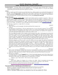
Affine transformations:
An affine transformation is of the form
⎛
f(
x ⎝
y
⎞ ⎛
⎠) =
⎝ a
b
c d
⎞
or
⎠ ·
⎛
⎝ x y
⎞ ⎛
⎠ +
⎝ e f
⎞
⎠
⎛
f(
x ⎝
y
⎞ ⎛
⎠) = ⎝
r cos(θ) −s sin(φ)
r sin(θ) s cos(φ)
⎞
⎠ ·
⎛
⎝ x y
⎞ ⎛
⎠ +
⎝ e f
⎞
⎠
• r and s are the scaling factors in the x and y directions resp.
• θ and φ measure rotation of horizontal and vertical lines resp.
• e and f measure horizontal and vertical translations resp.
It can be easily shown that:
• r 2 = a 2 + c 2 ,
• s 2 = b 2 + d 2 ,
• θ = arctan(c/a), and
• φ = arctan(−b/d).
✻
b
✻
✛
θ
a
c
✲
✛
d
φ
✲
❄
❄
2

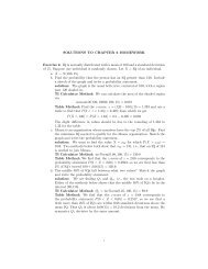
For example, shears are represented as follows:
B ′ A ′
✻
.....................
.....................
✻
.....................
.....................
..................... B
..................... B C
C
C
..................... .....................
✲
..................... .....................
′
✲
D
A
D
A
x ′ = x
y ′ = 2x + y
Shear in the y direction
x ′ = x + 2y
y ′ = y
Shear in the x direction
B ′
⎛
a ⎝
b
c d
⎞
⎠ =
⎛
⎝ 1 0
2 1
⎞
⎠
⎛
a ⎝
b
c d
⎞
⎠ =
⎛
⎝ 1 2
0 1
⎞
⎠
r = √ 5, s = 1 r = 1, s = √ 5
θ = 63.435, φ = 0 θ = 0, φ = −63.435
3

Finding IFS Rules from Images of Points
Given three non-collinear initial points p 1 = (x 1 , y 1 ), p 2 = (x 2 , y 2 ), p 3 =
(x 3 , y 3 ) and three image points q 1 = (u 1 , v 1 ), q 2 = (u 2 , v 2 ), q 3 = (u 3 , v 3 ) respectively.
Find an affine transformation T such that T (p 1 ) = q 1 , T (p 2 ) =
q 2 , and T (p 3 ) = q 3 .
Recall that,
⎛
T (
x ⎝
y
⎞ ⎛
⎠) =
⎝ a
b
c d
⎞ ⎛
⎠ ·
⎝ x y
⎞ ⎛
⎠ +
⎝ e f
⎞
⎠
Now Using p 1 , p 2 , p 3 and their images we arrive at the following six equations
in six unknowns:
ax 1 + by 1 + e = u 1
cx 1 + dy 1 + f = v 1
ax 2 + by 2 + e = u 2
cx 2 + dy 2 + f = v 2
ax 3 + by 3 + e = u 3
cx 3 + dy 3 + f = v 3
This system has a unique solution if and only if the points p 1 , p 2 , and p 3
are noncollinear.
4

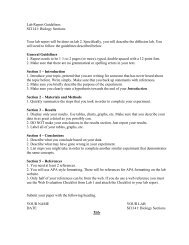
Example: The Seirpinski Triangle
1 .....................
.........................................
.........................................
.5, 0, 0, .5, .........................................
0, .5
.....................
.....................
.....................
.....................
.........................................
.........................................
.5, 0, 0, .5, .5, 0
.........................................
.........................................
.....................
0
.5, 0, 0, .5, 0, 0
1
The IFS for the Seirpinski triangle is {T 1 , T 2 , T 2 } where
⎛
T 1 (
x ⎝
y
⎛
T 2 (
x ⎝
y
⎛
T 3 (
x ⎝
y
⎞ ⎛
⎠) =
.5 0 ⎝
0 .5
⎞ ⎛
⎠) =
.5 0 ⎝
0 .5
⎞ ⎛
⎠) =
.5 0 ⎝
0 .5
⎞
⎠ ·
⎞
⎠ ·
⎞
⎠ ·
⎛
⎝ x y
⎛
⎝ x y
⎛
⎝ x y
⎞
⎠ +
⎞
⎠ +
⎞
⎠ +
⎛
⎝ 0 0
⎛
⎝ .5 0
⎛
⎝ 0
.5
⎞
⎠
⎞
⎠
⎞
⎠
http://smccd.net/accounts/hasson/fract.html
5

Example: The Seirpinski Carpet
2
3
1
3
✻
1 . . V I V II V III
.....................
.....................
.....................
IV
V
.....................
.....................
.....................
I II III
0 .....................
.....................
.....................
0
1
1
3
2
3
✲
The IFS for the Seirpinski carpet is {T 1 , T 2 , T 3 , T 4 , T 5 , T 6 , T 7 , T 8 } where
⎛
T 1 (
x ⎝
y
⎛
T 2 (
x ⎝
y
⎛
T 3 (
x ⎝
y
⎛
T 4 (
x ⎝
y
⎛
T 5 (
x ⎝
y
⎛
T 6 (
x ⎝
y
⎛
T 7 (
x ⎝
y
⎛
T 8 (
x ⎝
y
⎞ ⎛
⎠) =
.333 0
⎝
0 .333
⎞ ⎛
⎠) =
..333 0
⎝
0 .333
⎞ ⎛
⎠) =
.333 0
⎝
0 .333
⎞ ⎛
⎠) =
.333 0
⎝
0 .333
⎞ ⎛
⎠) =
.333 0
⎝
0 .333
⎞ ⎛
⎠) =
.333 0
⎝
0 .333
⎞ ⎛
⎠) =
.333 0
⎝
0 .333
⎞ ⎛
⎠) =
.333 0
⎝
0 .333
⎞
⎞
⎠ ·
⎠ ·
⎞
⎠ ·
⎞
⎠ ·
⎞
⎠ ·
⎞
⎠ ·
⎞
⎠ ·
⎞
⎠ ·
⎛
⎛
⎝ x y
⎝ x y
⎛
⎝ x y
⎛
⎝ x y
⎛
⎝ x y
⎛
⎝ x y
⎛
⎝ x y
⎛
⎝ x y
⎞
⎞
⎠ +
⎠ +
⎞
⎠ +
⎞
⎛
⎛
⎝ 0 0
⎞
⎠
⎝ .333 0
⎛
⎠ + ⎝
⎞
⎠ +
⎞
⎝ .666 0
⎛
⎛
⎠ + ⎝
⎞
⎠ +
⎞
⎠ +
0
.333
⎝ .666
.333
⎛
⎛
0
.666
⎝ .333
.666
⎛
⎝ .666
.666
⎞
⎠
⎞
⎠
⎞
⎠
⎞
⎠
⎞
⎠
⎞
⎠
⎞
⎠
6

Example: A simple tree
✻
........... (5,...........
20)
...........
...........
(15, ...........
20)
...........
.
.5, −.5, .5, .5, . 5, 5
...........
.
...........
. . .5, .5, −.5, . .5, 5, 15
(5, 15) (15, 15)
(0, 15)
........... ...........
...........
...........
...........
...........
.
(20, 15)
.
...........
.
...........
. . .
........... ...........
...........
...........
...........
...........
.
(10, 10)
.
...........
.
...........
. . . −10 < x < 30
0 < y < 40
........... ...........
...........
...........
...........
...........
.
.
...........
.
...........
. . .
T runk 0, 0, 0, .333, 10, 0
........... ...................
...................... ..........
........... ..........
✲
(10, 0)
The IFS for the tree is {T 1 , T 2 , T 2 } where
⎛
T 1 (
x ⎝
y
⎛
T 2 (
x ⎝
y
⎛
T 3 (
x ⎝
y
⎞ ⎛
⎠) = ⎝
⎞ ⎛
⎠) = ⎝
.5 .5
−.5 .5
.5 −.5
.5 .5
⎞ ⎛
⎠) =
0 0
⎝
0 .333
⎞
⎠ ·
⎞
⎠ ·
⎞
⎠ ·
⎛
⎝ x y
⎛
⎝ x y
⎛
⎝ x y
⎞
⎠ +
⎞
⎠ +
⎞
⎠ +
⎛
⎝ 5
15
⎛
⎝ 5 5
⎛
⎝ 10 0
⎞
⎠
⎞
⎠
⎞
⎠
http://alumnus.caltech.edu/ chamness/equation/equation.html
http://smccd.net/accounts/hasson/fract.html
7

Demonstrate some of the java applets at
http://classes.yale.edu/fractals/Software/Software.html
Discuss the IFS for the Fern.
Discuss the IFS for the mountain range.
Discuss the IFS for the Wave.
8

Iterated Function Systems:
An Iterated Function System in R 2 is a collection {F 1 , F 2 , . . . , F N } of contraction
mappings on R 2 . (F i is a contraction mapping if given x, y then
d(F i (x), F i (y)) ≤ s d(x, y) where 0 ≤ s < 1)
The Collage Theorem says that there is a unique nonempty compact
subset A ⊂ R 2 called the attractor such that
A = F 1 (A) ∪ F 2 (A) ∪ . . . ∪ F N (A)
Sketch of Proof:
Given a complete metric space X, let H(X) be the collection of nonempty
compact subsets of X. Given A and B in H(X) define d(A, B) to be the
smallest number r such that each point of in A is within r of some point
in B and vice versa. If X is complete so is H(X).
A = [0, 3]
B = [2, 4]
2 3 4
0 1 2 3
d(A, B) = 2
Given an IFS on X, define G : H(X) → H(X) by
G(K) = F 1 (K) ∪ . . . ∪ F N (K)
If each F i is a contraction then so is G. The contraction mapping theorem
says that a contraction mapping on a complete space has a unique fixed
point. Hence there is A ∈ H(X) such that
G(A) = A = F 1 (A) ∪ F 2 (A) ∪ . . . ∪ F N (A)
Given K 0 ⊂ R 2 , let K n = G n (K 0 ). Then
d(A, K n ) ≤ sn d(K 0 , G(K 0 ))
1 − s
Hence K n is a very good approximation of A for large enough n.
9

To understand the previous result note that:
d(A, K 0 ) = d( n→∞
lim K n , K 0 )
= n→∞
lim d(K n , K 0 )
≤ n→∞
lim d(K 0 , K 1 ) + d(K 1 , K 2 ) + · · · + d(K n−1 , K n )
≤ n→∞
lim d(K 0 , K 1 ) + sd(K 0 , K 1 ) + · · · + s n−1 d(K 0 , K 1 )
1
≤
1 − s d(K 0, K 1 )
Hence,
d(A, K 1 ) ≤ 1
1 − s d(K 1, K 2 ) ≤ s
1 − s d(K 0, K 1 )
d(A, K 2 ) ≤ 1
1 − s d(K 2, K 3 ) ≤ s2
1 − s d(K 0, K 1 )
.
Deterministic Algorithm: (Slow!)
Given K 0 , let K n = G n (K 0 ). Now K n → A and n → ∞.
Random Algorithm: (Fast!)
Given Q 0 ∈ K 0 , let Q i+1 = F j (Q i ) where F j is chosen with probability
p j from all of the F i . Clearly Q i ∈ K i and for sufficiently large i, Q i is
arbitrarily close to some point in A.
Choose p i ∼ |detA i|
N∑
|detA i |
i=1
= |a id i − b i c i |
N∑
|a i d i − b i c i |
i=1
Geometrically, choose p i “proportional to F i .”
.
10

How do these algorithms work:
3 33
3 21
3 22
3 31
3 32
3 13
3 23
3 11
3 12
1 33
11
2 33
1 31
1 32
2 31
2 32
1 13
1 21
1 2
2 11
2 12
1 23
2 13
2 23
1 11
1 12
2
2 21
2 22