Matlab code for damping identification using energy ... - CFD4Aircraft
Matlab code for damping identification using energy ... - CFD4Aircraft
Matlab code for damping identification using energy ... - CFD4Aircraft

You also want an ePaper? Increase the reach of your titles
YUMPU automatically turns print PDFs into web optimized ePapers that Google loves.
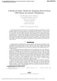
<strong>Matlab</strong> <strong>code</strong> <strong>for</strong> <strong>damping</strong> <strong>identification</strong> <strong>using</strong> <strong>energy</strong> balance<br />
technique<br />
The <strong>Matlab</strong> <strong>code</strong> provided per<strong>for</strong>ms the <strong>identification</strong> method described in [1] <strong>using</strong> the data<br />
obtained from experiments. This document contains a brief description of the theory and the<br />
instruction to use the <strong>code</strong> <strong>for</strong> the test cases presented.<br />
The <strong>energy</strong> method<br />
The equations of motion of a damped multi degree-of-freedom system can be written in the<br />
matrix <strong>for</strong>m<br />
Mẍ + Kx + Df(x, ẋ, ẍ) =g(t), (1)<br />
where M ∈ R n×n is the mass matrix, K ∈ R n×n is the stiffness matrix, D ∈ R n×n represents<br />
one of the possible <strong>damping</strong> matrices of coefficients multiplied by f(x, ẋ, ẍ) ∈ R n×1 , a function<br />
of displacements, velocities or accelerations. x ∈ R n×1 represents the vector of displacements<br />
and g(t) ∈ R n×1 the excitation input vector. Premultiplying by ẋ T andthenintegratingover<br />
time, the <strong>energy</strong> equation is obtained:<br />
∫<br />
t+T 1<br />
ẋ T Mẍdt +<br />
∫<br />
t+T 1<br />
ẋ T Kxdt +<br />
∫<br />
t+T 1<br />
ẋ T Df(x, ẋ, ẍ)dt =<br />
∫<br />
t+T 1<br />
ẋ T g(t)dt. (2)<br />
t<br />
t<br />
t<br />
t<br />
If the excitation <strong>for</strong>ce g(t) and the response x are periodic, the integration of conservative<br />
components of eq. (2) is zero over a full cycle of periodic motion. So if T is the period of g(t)<br />
and x, the sum of kinetic and potential <strong>energy</strong> over this period is zero:<br />
t+T ∫<br />
ẋ T Mẍdt +<br />
t+T ∫<br />
ẋ T Kxdt =0 (3)<br />
t<br />
t<br />
so eq. (2) becomes<br />
t+T ∫<br />
ẋ T Df(x, ẋ, ẍ)dt =<br />
t+T ∫<br />
ẋ T g(t)dt. (4)<br />
t<br />
t<br />
Eq. (4) represents the balance between the <strong>energy</strong> dissipated by the <strong>damping</strong> mechanisms<br />
on the left hand side of the equation and the <strong>energy</strong> input to the system on the right hand<br />
side. This equation is the base of the <strong>energy</strong>-balance <strong>identification</strong> method. There are no<br />
restrictions on f(x, ẋ, ẍ) andM and K are not required.<br />
Damping-pattern matrix approach<br />
The <strong>damping</strong>-pattern matrix approach is used to reduce the number of unknowns and to<br />
provide an easiest implementation in FEM models. A symmetric viscous <strong>damping</strong> matrix<br />
of a system with n degrees of freedom has (n 2 + n)/2 parameters to identify; this number<br />
can be considerably reduced by <strong>using</strong> in<strong>for</strong>mation and engineering knowledge of the system<br />
1
under study. Starting from eq. (4), in the case of viscous <strong>damping</strong> and considering the initial<br />
instant t=0, it becomes<br />
∫ T<br />
∫ T<br />
ẋ T Cẋ dt = ẋ T g(t) dt (5)<br />
0<br />
0<br />
where C is the viscous <strong>damping</strong> matrix, which can be written as<br />
C =<br />
p∑<br />
c i L i (6)<br />
i=1<br />
where L i ∈ R n×n is a matrix which indicates the location of the i th of p different viscous<br />
<strong>damping</strong> sources of amplitude c i .<br />
Figure 1: Absolute dashpot connecting DOF 2 to the ground<br />
In the case of an absolute dashpot connecting one degree of freedom (e.g. degree-of-freedom<br />
2, see figure 1) of the structure to the ground, L i takes the <strong>for</strong>m<br />
⎛<br />
⎞<br />
0 0 0 ··· 0<br />
0 1 0 ··· 0<br />
L i =<br />
0 0 0 ··· 0<br />
⎜<br />
⎝<br />
.<br />
. . . ..<br />
⎟<br />
0 ⎠<br />
0 0 0 0 0<br />
(7)<br />
Figure 2: Relative dashpot connecting DOF 1 to DOF 2<br />
In this case the pattern approach does not help the reduction of the number of unknowns,<br />
but helps a systematic procedure to define the <strong>damping</strong> sources in an automated way.<br />
2
In the case of a relative dashpots connecting two degrees of freedom together (e.g degree-offreedom<br />
1 and 2, see figure 2), L i takes the <strong>for</strong>m<br />
⎛<br />
⎞<br />
1 −1 0 ··· 0<br />
−1 1 0 ··· 0<br />
L i =<br />
0 0 0 ··· 0<br />
(8)<br />
⎜<br />
⎝<br />
.<br />
. . . ..<br />
⎟<br />
0 ⎠<br />
0 0 0 0 0<br />
which allows the reduction of the number of parameters to identify from 4 to 1. If the<br />
<strong>damping</strong> between two consecutive degrees of freedom is assumed to be the same <strong>for</strong> all the<br />
different couples (figure 3) representing, <strong>for</strong> example, the material <strong>damping</strong> between identical<br />
Figure 3: Identical relative dashpots connecting consecutive DOFs<br />
elements or similar connections or joints between parts of the structure, L i can take the <strong>for</strong>m<br />
⎛<br />
⎞<br />
1 −1 0 ··· 0 0<br />
−1 2 −1 ··· 0 0<br />
0 −1 2 ··· 0 0<br />
L i =<br />
.<br />
⎜ . . . .. (9)<br />
−1 0<br />
⎟<br />
⎝ 0 0 0 −1 2 −1 ⎠<br />
0 0 0 0 −1 1<br />
reducing the number of non-zero unknowns, in a 10 degrees of freedom example, from 28 to<br />
1.<br />
Assuming p different possible configurations <strong>for</strong> the <strong>damping</strong> sources, the <strong>energy</strong> equation<br />
(5) can be arranged as<br />
c 1<br />
∫T<br />
0<br />
ẋ T L 1 ẋ dt + c 2<br />
∫T<br />
0<br />
ẋ T L 2 ẋ dt + ...+ c p<br />
∫T<br />
0<br />
ẋ T L p ẋ dt =<br />
∫ T<br />
0<br />
ẋ T g(t) dt (10)<br />
By exciting the structure with q excitations at different frequencies, different versions of<br />
eq. (10) are obtained and arranged in a matrix <strong>for</strong>m<br />
⎡<br />
⎤<br />
⎧<br />
⎫<br />
∫T 1<br />
∫T 1<br />
∫T 1<br />
ẋ T L 1 ẋ dt ... ẋ T L p ẋ dt<br />
⎧ ⎫ ẋ T g 1 (t) dt<br />
0<br />
0<br />
⎪⎨ c 1 ⎪⎬ ⎪⎨ 0<br />
⎪⎬<br />
. . .<br />
. =<br />
⎢ T<br />
⎣ ∫ q<br />
∫T q<br />
⎥ ⎪⎩ ⎪<br />
.<br />
(11)<br />
⎭<br />
⎦ c p ∫T q<br />
ẋ T L 1 ẋ dt ... ẋ T L p ẋ dt<br />
⎪⎩ ẋ T g q (t) dt ⎪⎭<br />
0<br />
0<br />
3<br />
0
or, in a more compact <strong>for</strong>m,<br />
Ac = e (12)<br />
Eq. (12) can be solved <strong>for</strong> vector c <strong>using</strong> least square techniques and <strong>for</strong>cing the non-negative<br />
definiteness of the identified <strong>damping</strong> matrix at the same time. When vector c is calculated,<br />
the full identified viscous <strong>damping</strong> matrix can be obtained from eq. (6)<br />
Experimental setup<br />
The experiment consists in an aluminium cantilever beam (660×40×4 mm) with several<br />
sources of <strong>damping</strong> attached at different locations (figure 4). The structure is excited with<br />
Figure 4: Experimental setup<br />
a shaker in degree-of-freedom 3 (figure 5) and accelerations are measured in ten different<br />
locations equally spaced along the length of the beam. The structure is excited with several<br />
Figure 5: Definition of the DOFs of the experiment and location of the shaker<br />
different single frequency excitations at frequencies close to the natural frequencies (where<br />
the <strong>damping</strong> is assumed to be more relevant) and the measured time histories are used to<br />
apply the <strong>identification</strong> method proposed.<br />
4
Analytical integration of experimental data<br />
A single frequency sinusoidal function has been used to curve-fit the experimental measurements<br />
in order to use an analytical integration of accelerations to obtain velocities and<br />
displacements and to obtain an analytical expression of the integrals present in eq. (11).<br />
Considering a single test with an excitation at frequency ω i , vector g i (t) takethe<strong>for</strong>m<br />
⎧<br />
⎪⎨<br />
g i (t) =<br />
⎪⎩<br />
0<br />
0<br />
g i (t)<br />
0<br />
0<br />
0<br />
0<br />
0<br />
0<br />
0<br />
⎫<br />
⎪⎬<br />
⎪⎭<br />
(13)<br />
The input is assumed to be perfectly sinusoidal, so the measurement of g i (t) from the <strong>for</strong>ce<br />
transducer is fit to a harmonic function (figure 6) as<br />
g i (t) =r i sin(ω i t)+s i cos(ω i t) (14)<br />
by estimating the two coefficients r i and s i <strong>using</strong> least squares technique.<br />
8<br />
6<br />
Measured<br />
Sine-fit<br />
4<br />
Force (N)<br />
2<br />
0<br />
−2<br />
−4<br />
−6<br />
0 0.001 0.002 0.003 0.004 0.005 0.006 0.007 0.008 0.009 0.01<br />
Time (s)<br />
Figure 6: Typical measured and sine-fit <strong>for</strong>ce<br />
5
The same procedure is used <strong>for</strong> the measurement from the ten accelerometers as<br />
⎧<br />
⎪⎨<br />
ẍ i (t) =<br />
⎪⎩<br />
ẍ 1i (t)<br />
ẍ 2i (t)<br />
ẍ 3i (t)<br />
ẍ 4i (t)<br />
ẍ 5i (t)<br />
ẍ 6i (t)<br />
ẍ 7i (t)<br />
ẍ 8i (t)<br />
ẍ 9i (t)<br />
ẍ 10i (t)<br />
⎫<br />
⎪⎬ ⎪⎨<br />
=<br />
⎪⎭<br />
⎧<br />
⎪⎩<br />
u 1i<br />
u 2i<br />
u 3i<br />
u 4i<br />
u 5i<br />
u 6i<br />
u 7i<br />
u 8i<br />
u 9i<br />
u 10i<br />
⎧<br />
⎫⎪ ⎬ ⎪⎨<br />
sin(ω i t)+<br />
⎪ ⎭<br />
⎪⎩<br />
v 1i<br />
v 2i<br />
v 3i<br />
v 4i<br />
v 5i<br />
v 6i<br />
v 7i<br />
v 8i<br />
v 9i<br />
v 10i<br />
⎫⎪ ⎬<br />
⎪ ⎭<br />
cos(ω i t) (15)<br />
or<br />
ẍ i (t) =u i sin(ω i t)+v i cos(ω i t) (16)<br />
so that velocities and displacements can be calculated by analytical integration as<br />
ẋ i (t) = 1 ω i<br />
(−u i cos(ω i t)+v i sin(ω i t)) (17)<br />
x i (t) =− 1 ω 2 i<br />
(u i sin(ω i t)+v i cos(ω i t)) (18)<br />
400<br />
300<br />
Measured<br />
Sine-fit<br />
200<br />
Acceleration ( m/s 2)<br />
100<br />
0<br />
−100<br />
−200<br />
−300<br />
0 0.001 0.002 0.003 0.004 0.005 0.006 0.007 0.008 0.009 0.01<br />
Time (s)<br />
Figure 7: Typical measured and sine-fit acceleration, DOF 1<br />
Using these expressions <strong>for</strong> <strong>for</strong>ces and velocities allows the analytical calculation of the integrals<br />
in eq. (11) avoiding problems due to numerical integration and with the precise measurement<br />
of the period T too. For the case where the single frequency excitation is at frequency<br />
ω i and all the measurements are fitted to harmonic functions at the same frequency only, the<br />
period T i is simply<br />
T i = 2π<br />
(19)<br />
ω i<br />
6
The integrals present in eq. (11) become<br />
and<br />
∫ T i<br />
ẋ T L j ẋ dt = π ωi<br />
3 (u iT L j u i + v iT L j v i ) (20)<br />
0<br />
∫ T i<br />
0<br />
ẋ T g 1 (t) dt = π ωi<br />
2 (v 3i r i − u 3i s i ) (21)<br />
All the elements to solve equation (12) are now ready and easily obtainable from real experiments.<br />
Test cases<br />
Several experiments have been per<strong>for</strong>med to validate the method proposed; the test cases<br />
presented include the undamped cantilever beam, the beam damped by an air dashpot and<br />
by a Coulomb friction device.<br />
Case 1: undamped system<br />
The first experiment is per<strong>for</strong>med on the undamped cantilever beam in order to estimate<br />
the offset <strong>damping</strong> due to the clamp, material <strong>damping</strong>, cables, air and everything else. The<br />
chosen parameterisation <strong>for</strong> the equivalent viscous <strong>damping</strong> matrix is obtained by ten absolute<br />
dashpots as eq. (7) <strong>for</strong> the ten degrees of freedom to identify local sources of <strong>damping</strong> plus a<br />
matrix as eq. (9) <strong>for</strong> taking into account <strong>for</strong> the dissipations between consecutive degrees of<br />
freedom (assumed equal) <strong>for</strong> a total of 11 parameters to estimate.<br />
Case 2: single air dashpot<br />
The air dashpot used in the experiment consists in a cylinder with a moving piston (figure 8)<br />
which <strong>for</strong>ces the air inside the cylinder to flow through an adjustable hole, allowing a variable<br />
<strong>damping</strong> coefficient. In this experiment the air dashpot has been set to a <strong>damping</strong> value of<br />
Figure 8: Air dashpot at DOF 4<br />
approximately 5 Ns/m, located at degree-of-freedom 8.<br />
7
Figure 9: Location of the air dashpot<br />
Case 3: coulomb friction<br />
In the following experiment, a calliper acting on the aluminium wing as shown in figure 10<br />
has been used. Different films of different materials can be applied to the wings and to the<br />
Figure 10: Coulomb friction device at DOF 9<br />
callipers to provide different combination of materials and different friction coefficient µ. The<br />
normal <strong>for</strong>ce is provided by the screw in the middle of the calliper and it can be measured by<br />
static tests by a dynamometer applied in the contact point. The tangential <strong>for</strong>ce is measured<br />
by a <strong>for</strong>ce transducer located between the calliper and the support. By knowing the normal<br />
and tangential <strong>for</strong>ce is it possible to calculate the Coulomb friction coefficient µ to compare to<br />
the one obtained by <strong>damping</strong> <strong>identification</strong>. The Coulomb friction device has been attached<br />
Figure 11: Location of the coulomb friction device<br />
to degree-of-freedom 6.<br />
8
Using the <strong>code</strong><br />
When the file “En Method.m” is run into <strong>Matlab</strong>, it will ask to select which case to open.<br />
The case files (*.zip) are compressed *.mat files which have to be uncompressed in order<br />
to be used. The *.mat files contain the measured accelerations of the ten accelerometers<br />
(accNdata) <strong>for</strong> the different excitations at frequencies (excfr), the time vector (timedata),<br />
the measured excitation <strong>for</strong>ces (<strong>for</strong>cedata) and some in<strong>for</strong>mation about the test case.<br />
After the selection of the file, the <strong>code</strong> will filter the data according to the band defined by the<br />
two variables “lowestfrequency” and “highestfrequency”. This filter became necessary when<br />
it was discovered that the standard accelerometers used were affected by a phase delay at low<br />
frequencies. Then, the acceleration and <strong>for</strong>ce measurements are fit to a harmonic function as<br />
described in the previous sections.<br />
At this point the <strong>code</strong> will ask if the plot of the approximated functions versus the original<br />
data has to be displayed. By clicking “Yes”, a few periods of each measurement will be displayed<br />
in separate plots (one <strong>for</strong> each degree of freedom) together with their approximations,<br />
in order to evaluate if the harmonic functions are sufficient to approximate the measured<br />
data.<br />
The next step is to define the <strong>damping</strong> pattern. In this example the chosen parameterisation<br />
<strong>for</strong> the equivalent viscous <strong>damping</strong> matrix is obtained by ten absolute dashpots in order<br />
to identify local sources of <strong>damping</strong> plus a matrix as eq. (9) <strong>for</strong> taking into account <strong>for</strong><br />
the dissipations between consecutive degrees of freedom (assumed equal), <strong>for</strong> a total of 11<br />
parameters to estimate.<br />
The matrix of integrals A and the <strong>energy</strong> vector e are then computed <strong>using</strong> eqs. (20) and<br />
(21) and the <strong>energy</strong> equation is simply solved <strong>using</strong> the command “lsqnonneg” <strong>for</strong>cing the<br />
non-negativeness of the <strong>damping</strong> parameters which guarantees the non-negative definitess of<br />
the viscous <strong>damping</strong> matrix defined by eq. (6) <strong>using</strong> the <strong>damping</strong> pattern just defined.<br />
A plot of the identified equivalent viscous <strong>damping</strong> matrix and a plot the <strong>energy</strong> contribution<br />
of each degree of freedom to the total dissipation of <strong>energy</strong> are then provided and the<br />
equivalent viscous <strong>damping</strong> matrix is saved in the variable “Cid”.<br />
9
Bibliography<br />
[1] M. Prandina, J.E. Mottershead, and E. Bonisoli. Damping <strong>identification</strong> in multiple<br />
degree-of-freedom systems <strong>using</strong> an <strong>energy</strong> balance approach. Journal of Physics: Conference<br />
Series, 181(012006), 2009.<br />
11