Multivariate Regression Trees for Analysis of Abundance Data

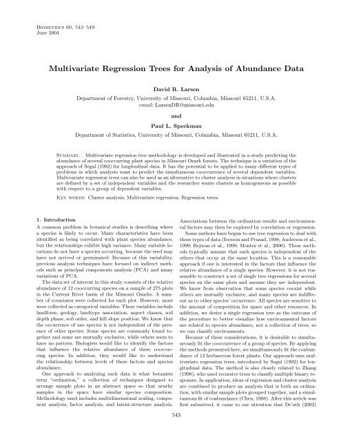
Biometrics 60, 543–549
June 2004
Multivariate Regression Trees for Analysis of Abundance Data
David R. Larsen
Department of Forestry, University of Missouri, Columbia, Missouri 65211, U.S.A.
email: LarsenDR@missouri.edu
and
Paul L. Speckman
Department of Statistics, University of Missouri, Columbia, Missouri 65211, U.S.A.
Summary. Multivariate regression tree methodology is developed and illustrated in a study predicting the
abundance of several cooccurring plant species in Missouri Ozark forests. The technique is a variation of the
approach of Segal (1992) for longitudinal data. It has the potential to be applied to many different types of
problems in which analysts want to predict the simultaneous cooccurrence of several dependent variables.
Multivariate regression trees can also be used as an alternative to cluster analysis in situations where clusters
are defined by a set of independent variables and the researcher wants clusters as homogeneous as possible
with respect to a group of dependent variables.
Key words: Cluster analysis; Multivariate regression; Regression trees.
1. Introduction
A common problem in botanical studies is describing where
a species is likely to occur. Many characteristics have been
identified as being correlated with plant species abundance,
but the relationships exhibit high variance. Many suitable locations
do not have a species occurring, because the seed may
have not arrived or germinated. Because of this variability,
previous analysis techniques have focused on indirect methods
such as principal components analysis (PCA) and many
variations of PCA.
The data set of interest in this study consists of the relative
abundance of 12 cooccurring species on a sample of 275 plots
in the Current River basin of the Missouri Ozarks. A number
of covariates were collected for each plot. However, most
were collected as categorical variables. These variables include
landform, geology, landtype association, aspect classes, soil
depth phase, soil order, and hill slope position. We know that
the occurrence of one species is not independent of the presence
of other species. Some species are commonly found together
and some are mutually exclusive, while others seem to
have no pattern. Biologists would like to identify the factors
that influence the relative abundance of these cooccurring
species. In addition, they would like to understand
the relationship between levels of these factors and species
abundance.
One approach to analyzing such data is what botanists
term “ordination,” a collection of techniques designed to
arrange sample plots in an abstract space so that nearby
samples in the space have similar species composition.
Methodology used includes multidimensional scaling, component
analysis, factor analysis, and latent-structure analysis.
543
Associations between the ordination results and environmental
factors may then be explored by correlation or regression.
Some authors have begun to use tree regression to deal with
these types of data (Iverson and Prasad, 1998; Anderson et al.,
1999; Rejwan et al., 1999; Montes et al., 2000). These methods
typically assume that each species is independent of the
others that occur at the same location. This is a reasonable
approach if one is interested in the factors that influence the
relative abundance of a single species. However, it is not reasonable
to construct a set of single tree regressions for several
species on the same plots and assume they are independent.
We know from observation that some species coexist while
others are mutually exclusive, and many species are indifferent
as to other species’ occurrence. All species are sensitive to
the amount of competition for space and other resources. In
addition, we desire a single regression tree as the outcome of
the procedure to better visualize how environmental factors
are related to species abundance, not a collection of trees, so
we can classify environments.
Because of these considerations, it is desirable to simultaneously
fit the cooccurrence of a group of species. By applying
the methods presented here, we simultaneously fit the coabundance
of 12 herbaceous forest plants. Our approach uses multivariate
regression trees, introduced by Segal (1992) for longitudinal
data. The method is also closely related to Zhang
(1998), who used recursive trees to classify multiple binary responses.
In application, ideas of regression and cluster analysis
are combined to produce an analysis that is both an ordination,
with similar sample plots grouped together, and a simultaneous
fit of coabundance (Chen, 1998). After this article was
first submitted, it came to our attention that De’ath (2002)

544 Biometrics, June 2004
simultaneously developed the same approach for marine
species in Australia.
In this article, we wish to show the similarities and differences
with single regression trees and the procedures commonly
used in fitting those trees. We restrict our partitioning
metric to deviance as it is the most common partitioning
metric in single tree regression. Moreover, the algorithm for
multivariate regression trees using deviance is efficient enough
to use cross-validation in selecting tree size.
1.1 Data Description
The data set is from a study designed to develop an ecological
site classification system for the Missouri Ozarks. This
project is part of an effort of the Missouri Resources Assessment
Partnership (MoRAP), and the data were collected on
275 plots in the summer of 1997. Plots were located in Shannon,
Carter, and Oregon counties of the southeastern Missouri
Ozarks. The aim of the survey was to identify relationships
between the vegetation (species presence and abundance) and
environmental variables (e.g., geology, soil type, and landform).
The independent variables are categorical; Table 1 gives
the number of observations by category. The variables are defined
as follows. Landtype association is a layer in a national
hierarchical classification system based on local climate, to-
Table 1
Independent categorical variables with the number
in each category
Variable Category N
Landtype association Current River Breaks 118
Current River Hills 76
Jack Fork, Eminence Breaks 81
Geology Roubidoux 86
Upper Gasconade 107
Lower Gasconade 55
Gunter 6
Eminence 15
Van Buren 6
Landform Summit 16
Shoulder ridge 24
Shoulder 16
Backslope 195
Bench 24
Aspect class Exposed 97
Neutral east 54
Neutral west 45
Protected 79
Phase Deep 226
Variable depth 49
Soil order Alfisol 104
Mollisol 9
None 72
Ultisol 90
Position Upper 90
Upper-middle 28
Middle 51
Lower-middle 28
Lower 61
None 18
Table 2
Dependent variables with the number of samples out of 275 in
which the species occurred. All other statistics are for the
samples in which the species occurred.
Variable N a ¯x Minimum Maximum
Aster patens 118 0.3019 0.01 3.0
Carex digitalis 100 0.4133 0.01 3.0
Desmodium glutinosum 101 3.361 0.01 10.0
Desmodium roundifolium 117 0.2244 0.01 3.0
Euphorbia corollata 122 0.1948 0.01 0.5
Lespedeza intermedia 130 0.2098 0.01 0.5
Monarda russeliana 125 0.4110 0.01 3.0
Panicum commutatum 133 0.2495 0.01 0.5
Phryma leptostachya 106 0.3160 0.01 3.0
Smilax bona-nox 101 1.0650 0.01 20.0
Smilax racemosa 125 0.3244 0.01 3.0
Vaccinium vacillans 195 3.3610 0.01 20.0
a Number of samples with this species present from the 275 samples.
All other statistics are for only the samples with the species present.
The data for these variables are numerical but grouped into six
categories (0, 0.01, 0.5, 3.0, 10.0, 20.0).
pography, geology, soil groups, and broad vegetation patterns
(Keys et al., 1995). Geology describes the surface geological
formations. The materials in the study area are of the Ordivician
and Cambrian Periods. Landform is a description of the
unit of land’s position in a landscape. The values are ordered
from the top of a ridge to the valley bottom. Aspect classes
are designed to characterize a location’s exposure to the sun.
“Exposed” designates locations with aspect with 160–250 ◦ azimuth,
“Neutral east” denotes aspects with 71–159 ◦ azimuth,
“Neutral west” denotes aspects with 251–339 ◦ azimuth, and
“Protected” denotes aspects with 340–70 ◦ azimuth. Phase describes
the character of the soil, either deep or variable depth
to bedrock. Soil order is the soil taxonomic order. Position is
the relative hill slope position.
Table 2 describes the presence and abundance of the dependent
variables. The dependent variables are numerical but
were grouped into six categories (0, 0.01, 0.5, 3.0, 10.0, 20.0).
While this convention may seem unusual to a biometrician, it
is typical of the type of data commonly collected by botanists.
Botanists are quite confident in their ability to discriminate
categorical differences, but uncomfortable in attempting to
estimate continuous variables even on a percentage scale. Because
of this propensity to collect categorical data, analysis
becomes a challenge. After exploring many options, we concluded
that an extension of tree regression to the multivariate
setting would provide an appropriate method to analyze data
of this type.
2. Multivariate Regression Trees
We assume that the reader is familiar with ordinary regression
tree methodology, and give a brief overview here.
In the classic CART (Classification Analysis and Regression
Tree) program of Breiman et al. (1984), a greedy search algorithm
is used to construct a binary tree in the independent
variables. The goal is to produce nodes as homogeneous
as possible with respect to the dependent variable. Consider
the multiple regression problem y i = f(x i1 , ..., x ip ) + ε i ,
i =1,..., n, where f is unknown and not easily parameterized,

Multivariate Regression Trees for Analysis of Abundance Data 545
x ij are known independent variables, and ε i are random error
terms with zero means. A node N is a subset of the indices
{1, ..., n}. The deviance of a node N is defined as
∑
D(N) = {y i − ȳ(N)} 2 , (1)
i∈N
where ȳ(N) is the mean over the observations in node N. The
algorithm is recursive. The root node consists of all observations.
At each stage, an attempt is made to divide a parent
node N into two child nodes, a “left” node N left and “right”
node N right , so as to minimize D(N left )+D(N right ). Splits of
the following forms are considered:
1. If x j is a continuous variable, consider all splits of the
form N left = {i ∈ N : x ij ≤ t}, N right = {i ∈ N : x ij >t}
for constants t.
2. If x j is ordinal, consider all splits as in (1).
3. If x j is categorical with L levels, consider all 2 L subsets.
We need not consider the empty set. Moreover to each
split into left and right subsets, there is an equivalent
split with the subsets reversed. Thus there are actually
2 L−1 − 1 splits to consider.
For each independent variable, all possible splits are considered
according to the appropriate rule, and the deviance for
the node following the split, D(N left )+D(N right ), is calculated.
The split with the smallest such deviance is saved as a
candidate. The candidate splits are calculated for each independent
variable, and the variables whose best split produces
the smallest deviance is the one selected to partition node
N. The algorithm proceeds recursively until no further splitting
is possible according to the predetermined criteria. Typically,
an a priori minimum node size is specified (e.g., 10),
or splitting stops when the deviance of a node drops below a
certain level, e.g., 1% of the deviance of the root node. The
tree formed by these rules generally overfits the data, and a
variety of strategies have been used to “prune” the tree.
Now consider a multivariate regression setting where more
than one dependent variable is observed, y ij , j = 1,..., r.
The object of multivariate regression is to estimate a functional
relationship between the set of independent variables
x i1 , ..., x ip and the dependent variables. With a linear regression
model and independent, multivariate normal distributions,
maximum likelihood estimation is well known to be
equivalent to performing a succession of univariate regressions
(Anderson, 1984). However, this strategy is not attractive for
regression trees, because there is no obvious way to combine
separate, distinct trees into a single one. We seek a single tree
that simultaneously is good for estimating the mean response
of several dependent variables. Thus it is natural to consider
an extension of the definition of the partitioning metric, deviance.
Let V N be a known r × r positive definite matrix
defined for node N, and let y i =(y i1 , ..., y ir ) t . The vector c
that minimizes
∑
(y i − c) t V −1
N (y i − c) (2)
is clearly
i∈N
ȳ(N) = 1
#N
∑
y i , (3)
i∈N
where #N denotes the number of observations in node N. If
V N is proportional to Var (y i ) for observations in node N,
∑
D(N) = {y i − ȳ(N)} t V −1
N {y i − ȳ(N)} (4)
i∈N
is a natural definition of the deviance of the node. With definition
(4) for deviance, the recursive algorithm proceeds as in
the univariate case with one modification. When splitting a
node by a categorical variable with L levels (case 3 above) in
univariate regression, it can be shown that one need to consider
only L − 1 subsets instead of all 2 L−1 − 1 theoretical
possibilities (Breiman et al., 1984). However, for multivariate
regression trees, all splits must be examined, essentially because
Euclidean space is not completely ordered for dimension
greater than one.
This approach corresponds to the method of Segal (1992).
In his application, the vector y i is a set of longitudinal data
on a single individual with covariance matrix proportional to
V N , which also depends on parameters estimated from the
data. Segal noted that taking V to be the sample covariance
matrix of the full set of dependent variables corresponds to
Hotelling’s T 2 -statistic. Zhang (1998) also investigated this
form of deviance (see h 2 in his terminology) for binary response
data.
2.1 Analysis Methods
A complete tree was fit to the data set using the previously
described methods. We took V to be the sample covariance
matrix for the full data set. The greedy algorithm for tree
building of Breiman et al. (1984) is analogous to forward selection
in regression terminology. To ensure inclusion of all
relevant explanatory variables, the tree-building rules are set
to construct a large tree, one which invariably overfits the
data. A procedure analogous to backward selection is then
used to “prune” the tree, i.e., remove some of the terminal
nodes.
A goodness-of-fit criterion of a tree T having terminal nodes
{N k }, say, is defined as
∑
D(T )=
D(N k ). (5)
all terminal nodes N k
If a tree T ′ is a subtree of T, clearly D(T ) ≤ D(T ′ ). The pruning
algorithm successively removes pairs of terminal nodes
corresponding to the split with the smallest decrease in deviance.
In other words, if T has terminal nodes {N k }, then
each pair, say {N 2j , N 2j+1 }, was the result of splitting a higher
node, say N j , with D(N j ) ≥ D(N 2j )+D(N 2j+1 ). All such
pairs of terminal nodes are examined, and the pair with the
smallest drop in deviance D(N j ) − D(N 2j ) − D(N 2j+1 )isremoved
to create a new subtree T ′ . (In principle, there could
be more than one pair with the smallest drop in deviance.
In that case, all such pairs would be dropped at the same
time.) The method is analogous to removing the least significant
variable in backward selection. The process is repeated
to create a nested set of trees T m ⊂ ··· ⊂ T 0 , where T 0 is the
full tree and T m is the tree consisting of only the root node.
To choose among this sequence of trees, Breiman et al.
(1984) proposed a cost-complexity measure for tree T,
D α (T )=D(T )+α size(T ), (6)

546 Biometrics, June 2004
where α is a suitably chosen cost-complexity parameter. For
fixed α, there is at least one tree that minimizes D α (T). Taking
α =2σ 2 corresponds to AIC. However, in practice AIC
seems to lead to overfitting, and there appears to be no suitable
theory for objectively choosing a good α. Conversely,
Breiman et al. (1984) showed that the sequence of trees minimizing
D α is nested, so it is possible to consider the nested
sequence as a function of α. (In the case of ties, more than
one pair of terminal nodes may be dropped at the same time.)
The deviance of the nested sequence is a decreasing function
of α.
Some form of cross-validation is commonly used to choose
an appropriate subtree. If a separate validation set is available,
we can use the sequence of trees to predict that set and
select the one that minimizes the deviance. More often, we
split the data set into subsets and use the subsets for validation.
Following Breiman et al. (1984) and the implementation
in S, we randomly split the data set into m approximately
equal subsets (typically m = 10). For each subset, a tree is
grown on the remaining data, the optimal nested sequence is
obtained, and the deviance of predictions is computed. The
results of the m validation runs are averaged to produce a
cross-validation score.
Because the subsets used for cross-validation are chosen
at random, the output of this cross-validation procedure is
random, and successive runs will produce different plots. In
addition, Breiman et al. (1984) noted that the actual tree chosen
by cross-validation is highly data dependent. Thus crossvalidation
is suggestive, but cannot be used for confirmatory
analysis. In our application, we are interested in a tree useful
for description purposes, so scientific insight as well as
cross-validation plays an important role in choosing an appropriately
sized tree.
2.2 Results
The full multivariate regression tree T 1 fit to the Missouri
Ozarks data had 44 nodes, some of which contained as few
as five observations. A plot of the full tree is displayed in
Figure 1. The labels for each node show the variable selected
for the split; the codes of the categories for the left node are
also shown. The numbers at each node denote the sizes of
the nodes, and the length of the vertical line segments are
proportional to the drop in deviance corresponding to the
split. The stacked bars under each node indicate the relative
proportion of the observations in each node that come from
each species in the dependent variables. Here the multivariate
nature of this procedure starts to become apparent.
Next cross-validation was applied to the full tree. After
examining several cross-validation graphs, we chose to use a
tree with three nodes. In our judgment, a three-node tree
vvrel2
dgrel2
astepate2
caredigi2
desmrotu2
euphcoro2
lespinte2
monaruss2
panicomm2
phrylept2
smilbona2
smilrace2
phase:a
aspc:abc
|
geo:a
5
lf:b
5
lta:a lta:b
aspc:a
lf:b
lta:ab
8 6 9 6
11
lf:e
aspc:a
lta:b
5 6 5
geo:d
geo:ce
aspc:ab
lta:b
pos:d
pos:bc
aspc:a
ord:a lf:bd
5 5
lta:a
lf:b pos:acd 9 9 5 pos:bc
pos:abcd
5 5
5
lf:b
5
7 5
6 8
6
8
geo:e
pos:ac pos:ac
geo:c ord:a
6 5
5 7
lta:a
5
8 6
pos:bd
lta:a
pos:abcd
geo:cd
pos:ac
6
lta:b geo:cd 7
6 7
ord:a
7 7
6
5 5
lf:acde
lta:b
5
7 6
Figure 1. Full tree for the 12 dependent variables. The labels indicate the variable on which the tree split and the letters
indicate the categories on the left split. The numbers are the number of observations at that node.

Multivariate Regression Trees for Analysis of Abundance Data 547
93.0 46.0 29.0 23.0 22.0 18.0 16.0 15.0 13.0 8.7 7.5 6.5 5.9 4.9 2.8
deviance
3200 3300 3400 3500 3600
1 10 20 30 40
Figure 2. Cross-validation of the full tree indicating a reduced tree size of 6.
size
was consistently close to the minimum deviance tree. Again,
cross-validation graph calculations are dependent on random
numbers so each graph is different. To correctly evaluate
cross-validation, a number of cross-validation graphs must
be viewed to determine the minimum deviance. An example
of the cross-validation graph is presented in Figure 2. The
three-node tree is very simple. Because the purpose of this
analysis is to describe the factors that indicate differences
among the species, a five-node tree was developed as well.
The pruning procedure was applied to the full tree to reduce
the tree to the best three- and five-node trees. A graphical
representation similar to Figure 1 of the pruned three-node
tree is presented in Figure 3 and of the pruned five-node tree
is presented in Figure 4. These figures, while fit with the dependent
variables transformed by the square root to account
for the fact that the original dependent data is proportional,
are displayed showing counts by terminal node for ease of
interpretation.
2.3 Discussion
Multivariate regression trees extend single regression tree
methods. In this article, we have endeavored to illustrate the
analogous components and point out the significant differences.
Multivariate regression trees are well suited to situations
where we would like to identify the factors and their
levels that minimize the variation within each species in a
node. The decision to select single or multivariate regression
trees is determined by the response of interest, i.e., a single
species response or the combined response of a group of
species. Multivariate trees are well suited to determining the
factors that most strongly influence the species group used
for the response variables.
We opted to use multivariate regression trees because we
could not assume that the cooccurring species on a set of plots
were independent. The response of the multivariate regression
tree is the combined differences of all species in the species
group. The trees should be expected to be different from single
regression trees developed on each species. They do, however,
illustrate the factors and levels of those factors that minimize
the deviance within the species group at a node.
One must keep in mind that the objective of this analysis
is to develop a tree that describes the factors that distinguish
differences in species cooccurrence. We felt that one multivariate
tree is much easier to interpret than the 12 species-specific
single trees. The decision between these methodologies is dependent
on the user objectives. If the user is most interested
in the cooccurrence of plant species a multivariate tree regression
should be the most appropriate. If it is the factors
effecting a single species occurrence, a single regression tree
should be the most appropriate.
It is generally known that tree regressions are poor at prediction
of new observations. Many methods have been developed
to address this problem such as bagging or random
forests (Ghattas, 2000; Breiman et al., 2001). However, since
the results of these procedures do not have simple tree structures,
they are not as attractive as the simple tree in our
classification application.
Our multivariate regression trees relate plant abundance to
landform, geology, soil phase, and landtype characteristics for
select plants in the Current River of the Missouri Ozarks. In
Figures 3 and 4, the first split is on aspect class. Aspect class is
a principle factor in the amount of solar radiation received at
the plot location and the amount of moisture available there.
The second-level split is soil phase. Soil phase has two classes,
deep soils, which make up most of the landscape, and variable

548 Biometrics, June 2004
vvrel2
dgrel2
astepate2
caredigi2
desmrotu2
euphcoro2
lespinte2
monaruss2
panicomm2
phrylept2
smilbona2
smilrace2
aspc:abc
|
phase:a
79
154 42
Figure 3. Tree pruned to three nodes. The labels are the variables on which the tree split and the letters indicate the
categories that are on the left split.
vvrel2
dgrel2
astepate2
caredigi2
desmrotu2
euphcoro2
lespinte2
monaruss2
panicomm2
phrylept2
smilbona2
smilrace2
aspc:abc
|
phase:a
geo:a
5 74
154
geo:e
12 30
Figure 4. Tree pruned to five nodes. The labels are the variables on which the tree split and the letters indicate the
categories that are on the left split.

Multivariate Regression Trees for Analysis of Abundance Data 549
depth soils, which have a much higher plant diversity because
they contain a variety of environments. The third-level splits
on geology, which describes the stratographic layers of the
surface bedrock.
We explored the issue of dependent variable weighting and
found it very hard to develop clear conclusions. We tried trees
developed on the raw data, the square root transformed data,
the square root transformed data weighted by the variance
vector, and the square root transformed data weighted by
the variance/covariance matrix. All these variations created
plausible trees. However, the structures and the order of the
variables varied by the method. In the end, we chose to transform
by the square root and weight by covariance because
of our initial concern about the codependence of the dependent
variables. Tree regression is a method that given the
dependent variable space makes splits using a single independent
variable that maximizes the deviance between the split
nodes. This is repeated on the end nodes until the end node
reaches a stopping criteria. The nature of this method does
not make full use of the data set but focuses on key factors. It
is typically applied to data sets that exhibit weak dependent–
independent variable relationships, and the main objective is
to identify factors that most strongly group the data of the
dependent variable. Weighting then depends on the aspect
of the dependent variable that one wants to emphasis in the
analysis.
The method presented here allows one to use tree regression
methodology on systems of correlated dependent variables.
The procedures and diagnostic methods are closely related
to those developed for single variable tree regression.
De’ath (2002) suggested several alternative diagnostic tools
that are very familiar to biologists. This methodology has the
potential to be useful for many different types of problems.
We believe that these methods provide a valuable resource to
researchers with nonstandard classification problems or who
want to predict nonindependent y’s simultaneously.
3. Implementation
We have written a program that runs in S, S-PLUS, or R
on Linux, Solaris, and Windows. The program contains code
to create the regression tree, and modifications of S code are
included to estimate an “optimal” tree by cross-validation
and plot the regression trees with the barplots for each node.
Because the function produces a standard “tree” object, many
of the tree functions work without modification. These are
available from the authors.
Acknowledgements
Jennifer Grabner for collecting the data, June-Hung Chen for
analysis work, and Missouri Resource Assessment Partnership
and Missouri Department of Conservation for funding
the data collection.
Résumé
Une méthode multivariée par arbres de régression est
développée et illustrée par une étude prédisant l’abondance de
plusieurs espèces sympatriques de plantes des forêts d’Ozark
(Missouri, USA). La technique dérive de l’approche de
Segal (1992) pour les données longitudinales. Elle est potentiellement
applicable à de nombreux types de problèmes, en
particulier ceux dans lesquels l’analyste cherche àprédire la
co-occurrence simultanée de plusieurs variables dépendantes.
Les arbres de régression multivariés peuvent aussi être utilisés
comme une alternative à l’analyse hiérarchique par clusters
dans les cas où les groupes sont définis par un ensemble de
variables indépendantes et où le chercheur souhaite obtenir
des groupes les plus homogènes possibles par rapport àun
groupe de variables dépendantes.
References
Anderson, T. W. (1984). An Introduction to Multivariate Statistical
Analysis, 2nd edition. New York: John Wiley and
Sons.
Anderson, D., Portier, K., Obreza, T., Collins, M., and Pitts,
D. (1999). Tree regression analysis to determine effects of
soil variability on sugarcane yields. Soil Science Society
of America Journal 63, 592–600.
Breiman, L. (2001). Random Forests. Available at http://oz.
berkley.edu/users/breiman.
Breiman, L., Friedman, J. H., Olshen, R. A., and Stone, C. J.
(1984). Classification and Tree Regression. Monterey,
California: Wadsworth and Brooks/Cole.
Chen, J.-H. (1998). Multivariate regression trees. Master’s
Thesis, University of Missouri-Columbia.
De’ath, G. (2002). Multivariate regression trees: A new technique
for modeling species–environmental relationships.
Ecology 83, 1105–1117.
Ghattas, B. (2000). Aggregation of classification trees. Revue
de Statistique Appliquee—CERESTA 48, 85–98.
Iverson, L. R. and Prasad, A. M. (1998). Predicting abundance
of 80 tree species following climate change in the
Eastern United States. Ecological Monographs 68, 465–
485.
Keys, J. E., Jr., Carpenter, C. A., Hooks, S., Koenig, F.,
McNab, W. H., Russell, W., and Smith, M. L. (1995).
Ecological units of the eastern United States—first approximation.
USDA Forest Service, Atlanta, Georgia.
Montes, N., Gauquelin, T., Badri, W., Zaoui, E. H., and
Bertaudiere, V. (2000). A non-destructive method for
estimating above-ground forest biomass in threatened
woodlands. Forest Ecology and Management 130, 37–
46.
Rejwan, C., Collins, N. C., Brunner, L. J., Shuter, B. J., and
Ridgeway, M. S. (1999). Tree regression analysis on nesting
habitat of smallmouth bass. Ecology 80, 341–348.
Segal, M. R. (1992). Tree-structured methods for longitudinal
data. Journal of the American Statistical Association 87,
407–418.
Zhang, H. (1998). Classification trees for multiple binary responses.
Journal of the American Statistical Association
93, 180–193.
Received July 2003. Revised October 2003.
Accepted November 2003.