Intro to Inverse Trig Functions
Intro to Inverse Trig Functions
Intro to Inverse Trig Functions

You also want an ePaper? Increase the reach of your titles
YUMPU automatically turns print PDFs into web optimized ePapers that Google loves.
<strong>Inverse</strong> <strong>Trig</strong> <strong>Functions</strong><br />
Previously in Math 130. . .<br />
DEFINITION 24.1. A function g is the inverse of the function f if<br />
1. g( f (x)) = x for all x in the domain of f<br />
2. f (g(x)) = x for all x in the domain of g<br />
In this situation g is denoted by f −1 and is called “ f inverse."<br />
The Key Fact on the Existence of <strong>Inverse</strong>s<br />
THEOREM 24.1. f has an inverse ⇐⇒ f is one-<strong>to</strong>-one ⇐⇒ f passes the HLT.<br />
The Graph of f −1<br />
Now suppose that y = f (x) has an inverse, f −1 (x) and assume that a is in the<br />
domain of f and that f (a) = b. Then using the definition of inverse:<br />
In other words<br />
or<br />
f (a) = b ⇐⇒ f −1 ( f (a)) = f −1 (b) ⇐⇒ a <strong>Inverse</strong> = f −1 (b).<br />
f (a) = b ⇐⇒ f −1 (b) = a<br />
(a, b) on the graph of f ⇐⇒ (b, a) is on the graph of f −1<br />
In other words, f and f −1 have their x and y coordinates switched. And because<br />
the x and y coordinates are switched.<br />
• Domain of f −1 = Range of f<br />
• Range of f −1 = Domain of f<br />
If f is one-<strong>to</strong>-one, we can obtain the graph of f −1 by interchanging the x and y<br />
coordinates. If we draw the diagonal line y = x and use it as a mirror, notice that<br />
the x and y axes are reflected in<strong>to</strong> each other across the line.<br />
This is just another way of saying that the x and y coordinates have been switched.<br />
So <strong>to</strong> obtain the graph of f −1 all we need <strong>to</strong> do is <strong>to</strong> reflect the graph of f in the<br />
diagonal line y = x, as shown <strong>to</strong> the right.<br />
<strong>Intro</strong>duction<br />
•.<br />
.<br />
. •.<br />
.<br />
.<br />
.<br />
.<br />
f<br />
.<br />
.<br />
.<br />
.<br />
•<br />
.<br />
.<br />
.<br />
f −1<br />
.<br />
.<br />
.<br />
.<br />
•<br />
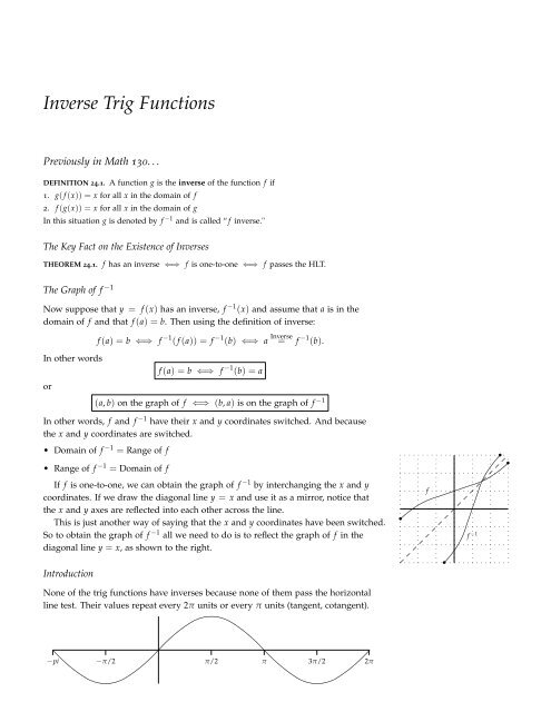
None of the trig functions have inverses because none of them pass the horizontal<br />
line test. Their values repeat every 2π units or every π units (tangent, cotangent).<br />
−pi −π/2 π/2 π 3π/2 2π<br />
.
2<br />
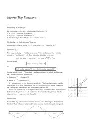
The <strong>Inverse</strong> Sine Function<br />
However, if we restrict the domain of the sine function (or any of the other trig<br />
functions) we can make the function one-<strong>to</strong>-one on the restricted interval. The<br />
figure on the left below shows sin x restricted <strong>to</strong> the interval [−π/2, π/2] where<br />
it is, indeed, one-<strong>to</strong>-one (passes HLT). So it has an inverse there, which we have<br />
graphed in red the figure on the right.<br />
1<br />
−π/2 π/2<br />
−1<br />
.<br />
−π/2 π/2<br />
.<br />
.<br />
.<br />
.<br />
.<br />
.<br />
.<br />
.<br />
.<br />
.<br />
.<br />
.<br />
.<br />
.<br />
.<br />
.<br />
.<br />
.<br />
.<br />
The inverse sine function is denoted by arcsin x. Your text uses sin −1 x, but most<br />
students find arcsin x less confusing, and that’s what we will generally use in this<br />
course. Since the domain and range of the sine and inverse sine functions are<br />
interchanged, we have<br />
• the domain of arcsin x is the range of the restricted sin x: [−1, 1].<br />
• the range of arcsin x is the domain of the restricted sin x: [−π/2, π/2]. This is<br />
very important. It says that the output of the inverse sine function is a number<br />
(an angle) between −π/2 and π/2.<br />
Notice since the arcsine function undoes the sine function, we get some familiar<br />
values: arcsin(−1) = −π/2 since sin(−π/2) = −1. Or arcsin(1/2) = π/6 since<br />
sin(π/6) = 1/2. Or arcsin( √ 3/2) = π/3 since sin(π/3) = √ 3/2.<br />
EXAMPLE 24.1. Normally when we calculate f −1 ( f (x)) we get x because the two functions<br />
undo each other. The same is true here, if the domain of sin x is appropriately<br />
restricted <strong>to</strong> [−π/2, π/2]. For example,<br />
arcsin(sin(π/4)) = arcsin( √ 2/2) = π/4.<br />
But if we take a value outside of the restricted domain [−π/2, π/2] of the sine function<br />
arcsin(sin(3π/4)) = arcsin( √ 2/2) = π/4.<br />
Or<br />
arcsin(sin(3π)) = arcsin(0) = 0.<br />
The two functions do not undo each other since the arcsine function can only return<br />
values (or angles) between −π/2 and π/2.<br />
The <strong>Inverse</strong> Cosine Function<br />
We can restrict the domains of the other trig functions so that they, <strong>to</strong>o, have inverses.<br />
The figure on the left below shows cos x restricted <strong>to</strong> the interval [0, π]<br />
where it is, indeed, one-<strong>to</strong>-one. So it has an inverse there, which we have graphed
math 130, calculus i 3<br />
in red the figure on the right.<br />
π<br />
. π<br />
.<br />
.<br />
.<br />
.<br />
.<br />
.<br />
.<br />
.<br />
.<br />
.<br />
.<br />
1<br />
1<br />
.<br />
.<br />
.<br />
.<br />
.<br />
.<br />
.<br />
−1 1 π<br />
−1 1 π<br />
.<br />
.<br />
.<br />
−1<br />
.<br />
−1<br />
.<br />
The inverse cosine function is denoted by arccos x. Since the domain and range of<br />
the cosine and inverse cosine functions are interchanged, we have<br />
• the domain of arccos x is the range of the restricted cos x: [−1, 1].<br />
• the range of arccos x is the domain of the restricted cos x: [0, π].<br />
EXAMPLE 24.2. Again we have <strong>to</strong> be careful about calculating the composites of these<br />
inverse functions. They are only inverses when the inputs are in the correct domains.<br />
For example,<br />
arccos(cos(π/4)) = arccos( √ 2/2) = π/4.<br />
But if we take a value outside of the restricted domain [0, π] of the cosine function<br />
Or<br />
arccos(cos(−π/4)) = arccos( √ 2/2) = π/4.<br />
arccos(cos(3π)) = arccos(−1) = π.<br />
The two functions do not always undo each other since the inverse cosine function can<br />
only return values between 0 and π.<br />
The <strong>Inverse</strong> Tangent Function<br />
The figure on the left below shows tan x restricted <strong>to</strong> the interval (−π/2, π/2)<br />
where it is, indeed, one-<strong>to</strong>-one. So it has an inverse there, which we have graphed<br />
in red the figure on the right.<br />
−π/2 π/2<br />
.<br />
.<br />
.<br />
.<br />
.<br />
.<br />
.<br />
.<br />
π/2<br />
.<br />
.<br />
.<br />
.<br />
.<br />
.<br />
.<br />
.<br />
.<br />
−π/2 . π/2<br />
.<br />
.<br />
.<br />
.<br />
.<br />
−π/2<br />
.<br />
.<br />
.<br />
.<br />
.<br />
.<br />
The inverse tangent function is denoted by arctan x. Since the domain and range of<br />
the tangent and inverse tangent functions are interchanged, we have<br />
• the domain of arctan x is the range of the restricted tan x: (−∞, ∞).
4<br />
• the range of arctan x is the domain of the restricted tan x: (−π/2, π/2).<br />
EXAMPLE 24.3. Again we have <strong>to</strong> be careful about calculating the composites of these<br />
inverse functions. They are only inverses when the inputs are in the correct domains.<br />
For example,<br />
arctan(tan(π/4)) = arctan(1) = π/4.<br />
But if we take a value outside of the restricted domain (−π/2, π/2) of the tangent<br />
function<br />
arctan(tan(3π/4)) = arctan(−1) = −π/4.<br />
Or<br />
arctan(tan(3π)) = arctan(0) = 0.<br />
The two functions do not always undo each other since the inverse tangent function<br />
can only return values between −π/2 and π/2.<br />
We will concentrate only on the the three inverse functions discussed above. I<br />
will leave it <strong>to</strong> you <strong>to</strong> read about the other inverse trig functions in your text.<br />
Evaluation Using Triangles<br />
Drawing appropriate right triangles can help evaluate complicated expressions<br />
involving the inverse trig functions.<br />
EXAMPLE 24.4. Evaluate cos(arcsin x).<br />
SOLUTION. Remember that arcsin x = θ where θ is just the angle whose sine is x. We<br />
want the cosine of this same angle. So let’s draw a right triangle with angle θ whose<br />
sine is x. Since the sine function is opp<br />
hyp we can use the triangle below.<br />
1<br />
x<br />
θ<br />
.<br />
x 2 + y 2 = 1 ⇒ y = √ 1 − x 2 .<br />
y<br />
Notice sin θ =<br />
1 x = x. So arcsin x = θ. (θ is the angle whose sine is x.) So<br />
cos(arcsin x) = cos(θ) = y √<br />
1 − x<br />
1 = 2<br />
= √ 1 − x<br />
1<br />
2 .<br />
EXAMPLE 24.5. Evaluate sec(arctan x).<br />
SOLUTION. This time we draw a triangle whose tangent is x.<br />
z<br />
x<br />
So<br />
.<br />
θ<br />
1<br />
z 2 = 1 2 + x 2 ⇒ z = √ 1 + x 2 .<br />
sec(arctan x) = sec(θ) = z 1 = √ 1 + x 2 .<br />
EXAMPLE 24.6. Evaluate sin(arccos 2/5).<br />
SOLUTION. This time we draw a triangle whose cosine is 2/5.<br />
5<br />
x<br />
So<br />
.<br />
θ<br />
2<br />
2 2 + x 2 = 5 2 ⇒ x = √ 5 2 − 2 2 = √ 21.<br />
sin(arccos 2/5) = sin(θ) = x 5 = √<br />
21<br />
5 .<br />
YOU TRY IT 24.1. Evaluate sin(arctan x) and cos(arcsin 3/4)).
math 130, calculus i 5<br />
Derivatives of arcsin x and arctan x<br />
Surprisingly, it is relatively easy <strong>to</strong> determine the derivatives of the inverse trig<br />
functions, assuming that they are differentiable. We will use implicit differentiation<br />
(really just the chain rule in disguise) just as we did when we figured out the<br />
derivative of ln x.<br />
Let’s first determine the derivative of y = arcsin x for − π 2 ≤ x ≤ π 2<br />
. We want <strong>to</strong><br />
find dy<br />
dx<br />
. First apply the inverse:<br />
y<br />
= arcsin x<br />
sin(y) = sin(arcsin x) = x.<br />
Now take the derivative using implicit differentiation on the left:<br />
D x [sin(y)] = D x [x]<br />
cos(y) dy<br />
dx = 1<br />
Solve for dy<br />
dx .<br />
dy<br />
dx = 1<br />
cos(y) = 1<br />
cos(arcsin x)<br />
But in Example 24.4 we found that cos(arcsin x) = √ 1 − x 2 so we have<br />
That is<br />
dy<br />
dx = 1<br />
cos(arcsin x) = 1<br />
√ .<br />
1 − x 2<br />
d<br />
dx (arcsin x) = 1<br />
√<br />
1 − x 2 .<br />
The derivative of y = arctan x for − π 2<br />
< x < π 2<br />
is determined in a similar<br />
fashion. We want <strong>to</strong> find dy<br />
dx<br />
. First apply the inverse:<br />
y = arctan x<br />
tan(y) = tan(arctan x) = x.<br />
Now take the derivative using implicit differentiation on the left:<br />
D x [tan(y)] = D x [x]<br />
sec 2 (y) dy<br />
dx = 1<br />
Solve for dy<br />
dx .<br />
dy<br />
dx = 1<br />
sec 2 (y) = 1<br />
sec 2 (arctan x)<br />
But in Example 24.5 we found that sec(arctan x) = √ 1 + x 2 so we have sec 2 (arctan x) =<br />
1 + x 2 . Therefore<br />
dy<br />
dx = 1<br />
sec 2 (arctan x) = 1<br />
1 + x 2 .<br />
That is<br />
d<br />
1<br />
(arctan x) =<br />
dx 1 + x 2 .<br />
YOU TRY IT 24.2 (Extra Credit). Determine the formula for the derivative of arccos x using the<br />
method above. Show your work.<br />
Keep going and find the derivatives of the remaining three inverse trig functions. Again<br />
show your work.
6<br />
Chain Rule Versions<br />
The chain rule versions of both derivative formulas are:<br />
d<br />
dx (arcsin u) = 1 du<br />
√<br />
1 − u 2 dx<br />
d<br />
1 du<br />
(arctan u) =<br />
dx 1 + u 2 dx<br />
EXAMPLE 24.7. Let’s use these formulas <strong>to</strong> find the derivatives of the following:<br />
d<br />
dx (arctan 1<br />
e3x ) =<br />
1 + (e 3x ) 2 · 3e3x = 3e3x<br />
1 + e 6x . (u = e3x )<br />
d<br />
dx (arcsin 3x2 ) =<br />
1<br />
√<br />
1 − (3x 2 ) 2 · 6x =<br />
6x<br />
√<br />
1 − 9x 4 . (u = 3x2 )<br />
d<br />
dx (earctan 3x ) = e arctan 3x 1 3earctan<br />
3x<br />
· 3 =<br />
1 + 9x2 1 + 9x 2 .<br />
d<br />
dx (sin 2x arctan 5x2 ) = 2 cos 2x arctan 5x 2 + sin 2x ·<br />
= 2 cos 2x arctan 5x 2 +<br />
10x sin 2x<br />
1 + 25x 4 .<br />
1<br />
1 + 25x 4 · 10x<br />
d<br />
dx (ln | arcsin 3x|) = 1<br />
arcsin 3x · 1<br />
√ · 3 = 3<br />
1 − 9x 2 (arcsin 3x) √ 1 − 9x . 2<br />
D x (| arcsin(ln 3x)) =<br />
1<br />
√ · 1<br />
1 − [ln(3x)] 2 3x · 3 = 1<br />
x √ 1 − [ln(3x)] . 2<br />
(u = ln(3x))<br />
YOU TRY IT 24.3. Find the derivatives of these functions:<br />
d<br />
dx arctan(6x2 )] =<br />
d<br />
dx [arcsin(√ x)] =<br />
d<br />
dx [arctan(e2x ] =<br />
d<br />
[arcsin(arcsin x)] =<br />
dx<br />
d<br />
d<br />
[arctan(ln |6x|)] =<br />
dx<br />
dx [arcsin(6esin x )] =<br />
d<br />
dx (e2 arcsin x2 ) =<br />
d<br />
dx [(arcsin 2x)(tan 5x2 )] =<br />
d<br />
dx (ln | arctan ex4 +1 |) =<br />
The answers are on the last page (on line) of this section.
math 130, calculus i 7<br />
Logarithmic Differentiation<br />
There are still types of functions that we have not tried <strong>to</strong> differentiate yet. Sometimes<br />
we can make use of our existing techniques and clever algebra <strong>to</strong> find<br />
derivatives of very complicated functions. Logarithmic differentiation refers <strong>to</strong><br />
the process of first taking the natural log of a function y = f (x), then solving for<br />
the derivative dy . On the surface of it, it would seem that logs would only make a<br />
dx<br />
complicated function more complicated. But remember that logs turn powers in<strong>to</strong><br />
products and products in<strong>to</strong> sums. That’s the key.<br />
Let’s look at the Extra Credit problem from Exam II <strong>to</strong> illustrate the idea.<br />
EXAMPLE 24.8. Use the chain rule and implicit differentiation along with logs <strong>to</strong> find<br />
the derivative of y = f (x) = x x .<br />
SOLUTION. We begin by taking the natural log of both sides and simplifying using<br />
log properties.<br />
ln y = ln x x Powers<br />
= x ln x.<br />
Remember we want <strong>to</strong> find dy , so take the derivative of both sides (implicitly on the<br />
dx<br />
left).<br />
d d<br />
(ln y) =<br />
dx dx (x ln x) ⇒ 1 y · dy<br />
dx = 1 · ln x + x · 1<br />
x = ln(x) + 1<br />
dy Solve<br />
= y[ln(x) + 1]<br />
dx<br />
dy Substitute<br />
= x x [ln(x) + 1]<br />
dx<br />
In other words, we have shown that<br />
Here are a couple more.<br />
EXAMPLE 24.9. Find the derivative of y = (1 + x 2 ) tan x .<br />
d<br />
dx (xx ) = x x [ln(x) + 1]. Neat! Easy!<br />
SOLUTION. Take the natural log of both sides and simplify using log properties.<br />
ln y = ln(1 + x 2 ) tan x Powers<br />
= tan x ln(1 + x 2 ).<br />
Take the derivative of both sides (implicitly on the left) and solve for dy<br />
dx .<br />
d d<br />
(<br />
)<br />
(ln y) = tan x ln(1 + x 2 )<br />
dx dx<br />
1<br />
y · dy<br />
dx = sec2 x ln(1 + x 2 ) + tan x ·<br />
dy Solve<br />
= y<br />
dx<br />
2x<br />
1 + x 2<br />
[<br />
]<br />
sec 2 x ln(1 + x 2 2x tan x<br />
) +<br />
1 + x 2<br />
[<br />
]<br />
dy Substitute<br />
= ln(1 + x 2 ) tan x sec 2 x ln(1 + x 2 2x tan x<br />
) +<br />
dx<br />
1 + x 2<br />
So d (ln(1 + x 2 ) tan x) [<br />
]<br />
= ln(1 + x 2 ) tan x sec 2 x ln(1 + x 2 2x tan x<br />
) +<br />
dx<br />
1 + x 2 . Not bad!<br />
EXAMPLE 24.10. Find the derivative of y = (ln x) x3 .<br />
SOLUTION. Be careful. This function is NOT the same as ln(x x3 ) which would equal<br />
x 3 ln x. Instead, take the natural log of both sides and simplify using log properties.<br />
ln y = ln(ln x) x3 Powers<br />
= x 3 ln(ln x).<br />
Take the derivative of both sides (implicitly on the left) and solve for dy<br />
dx .<br />
Do you see the difference when compared<br />
<strong>to</strong> ln(x x3 )
8<br />
1<br />
y · dy<br />
dx = 3x2 ln(ln x) + x 3 ·<br />
1<br />
ln x · 1<br />
x<br />
[3x 2 ln(ln x) + x3<br />
x ln x<br />
1<br />
y · dy Solve<br />
= y<br />
dx<br />
[<br />
dy Substitute<br />
= (ln x) x3 3x 2 ln(ln x) +<br />
dx<br />
]<br />
]<br />
x3<br />
x ln x<br />
Logs can also be used <strong>to</strong> simplify products and quotients.<br />
EXAMPLE 24.11. Find the derivative of y = (x2 − 1) 5√ 1 + x 2<br />
x 4 .<br />
+ 4<br />
SOLUTION. Use logarithmic differentiation <strong>to</strong> avoid a complicated quotient rule<br />
derivative Take the natural log of both sides and then simplify using log properties.<br />
(<br />
(x 2 − 1) 5√ )<br />
1 + x 2<br />
ln y = ln<br />
x 4 + 4<br />
Log Prop<br />
= ln(x 2 − 1) 5 + ln(1 + x 2 ) 1/2 − ln(x 4 + 4)<br />
Log Prop<br />
= 5 ln(x 2 − 1) + 1 2 ln(1 + x2 ) − ln(x 4 + 4).<br />
Take the derivative of both sides and solve for dy<br />
dx .<br />
1<br />
y · dy<br />
dx =<br />
dy Solve<br />
= y<br />
dx<br />
10x<br />
x 2 − 1 +<br />
[ 10x<br />
x 2 − 1 +<br />
x<br />
1 + x 2 − 4x3<br />
x 4 + 4<br />
x<br />
1 + x 2 − 4x3<br />
x 4 + 4<br />
dy Substitute (x<br />
=<br />
2 − 1) 5√ 1 + x 2<br />
dx<br />
x 4 + 4<br />
]<br />
[ 10x<br />
x 2 − 1 +<br />
x<br />
]<br />
1 + x 2 − 4x3<br />
x 4 + 4<br />
That would have been a real mess <strong>to</strong> do with the quotient rule (which would also<br />
require the product rule and the chain rule).<br />
Problems<br />
The following questions will be on the lab <strong>to</strong>morrow or are future WebWorK problems. Get<br />
a head start.<br />
1. Find the derivatives of the following functions. Use logarithmic differentiation where<br />
helpful.<br />
(a) y = (sin x) x (b) y = x sin x (c) (sin x) sin x<br />
(<br />
(d) (arcsin x) x2 (e) 1 + 1 ) x<br />
x<br />
2. Find the derivatives of these functions using the derivative formula for a general exponential<br />
function that we developed before Exam II. (See Theorem 3.18 on page 194).<br />
(a) 5 · 6 x (b) 2 x cot x (c) x π + π x (d) x 4 · 4 x<br />
(e) For which values of x does x 4 · 4 x have a horizontal tangent?
math 130, calculus i 9<br />
Answers.<br />
0. Answers <strong>to</strong> you try it 24.3 .<br />
d<br />
dx (arctan(6x2 )) =<br />
1<br />
12x<br />
d<br />
· 12x =<br />
1 + 36x4 1 + 36x 4 dx (arcsin(√ x)) =<br />
1<br />
√ · 1<br />
1 − x 2 · x−1/2 =<br />
1<br />
2 √ x √ 1 − x<br />
d<br />
dx (arctan(e2x )) =<br />
2e2x<br />
d<br />
1 + e 4x dx (arcsin(arcsin x)) = 1<br />
√ ·<br />
1 − (arcsin x) 2<br />
1<br />
√<br />
1 − x 2<br />
d<br />
dx [arctan(ln |6x|)] = 1<br />
1 + (ln |6x|) 2 · 1<br />
6x · 6 = 1<br />
x[1 + (ln |6x|) 2 ] .<br />
d<br />
dx (arcsin(6esin x )) =<br />
1<br />
√<br />
1 − (6e sin x ) 2 · (6esin x )(cos x) =<br />
6 cos xesin<br />
x<br />
√<br />
1 − (6e sin x ) 2<br />
d<br />
dx (e2 arcsin x2 ) = (e 2 arcsin 1<br />
x2 4xe2 arcsin x2<br />
) · 2 · √ · 2x = √<br />
1 − (x 2 ) 2 1 − x 4<br />
d<br />
dx [arcsin 2x(tan 2 tan 5x2 5x2<br />
)] = √ + (arcsin 2x)10x 1 − 4x 2 sec2 (5x 2 )<br />
d<br />
dx (ln | arctan ex4 +1 |) =<br />
1<br />
arctan e x4 +1 ·<br />
1<br />
1 + (e x4 +1 ) 2 · ex4 +1 · 4x 3 =<br />
4x 3 e x4 +1<br />
(arctan e x4 +1 )(1 + e 2x4 +2 )<br />
1. (a) ln y = ln(sin x) x = x ln(sin x) ⇒ 1 y · dy<br />
x cos x<br />
= ln(sin x) + ⇒<br />
dy<br />
dx<br />
sin x dx =<br />
(sin x) x (ln(sin x) + x cot x).<br />
(b) ln y = ln x sin x = sin x ln x ⇒ 1 y · dy<br />
dx = cos x ln x + (sin x) 1 x ⇒ dy (<br />
dx = xsin x cos x ln x + sin x )<br />
.<br />
x<br />
(c) ln y = ln(sin x) sin x = sin x ln(sin x) ⇒ 1 y · dy<br />
cos x<br />
= cos x ln(sin x) + (sin x)<br />
dx sin x ⇒ dy<br />
dx =<br />
(sin x) sin x cos x[ln(sin x) + 1].<br />
(d) ln y = ln(arcsin x) x2 = x 2 ln(arcsin x) ⇒ 1 y · dy<br />
dx = 2x ln(arcsin x) + 1<br />
x2<br />
(<br />
)<br />
arcsin x<br />
dy<br />
dx = (arcsin x x)x2 2x ln(arcsin x) +<br />
2<br />
(arcsin x) √ .<br />
1 − x 2<br />
(e) ln y = ln<br />
(<br />
1 + 1 ) x (<br />
= x ln 1 + 1 )<br />
⇒ 1 x x y · dy<br />
1<br />
y · dy (1<br />
dx = ln + 1 x<br />
(<br />
1 + 1 ) x [<br />
ln<br />
x<br />
(<br />
1 + 1 x<br />
)<br />
−<br />
)<br />
−<br />
(<br />
x<br />
1<br />
(x + 1)<br />
dx = ln (1 + 1 x<br />
1<br />
) ⇒ 1<br />
1 + 1 y · dy (1<br />
dx = ln + 1 x<br />
x<br />
]<br />
.<br />
)<br />
+ x ·<br />
)<br />
−<br />
1<br />
(<br />
1 + 1 x<br />
1<br />
√<br />
1 − x 2 ⇒<br />
) · −1<br />
x 2<br />
1<br />
(x + 1) ⇒ dy<br />
dx =<br />
2. (a)<br />
d<br />
dx [5 · 6x ] = 5 · 6 x ln 6 = 5 ln 6(6 x ).<br />
(b)<br />
d<br />
dx [2x cot x] = 2 x ln 2 cot x − 2 x csc 2 x = 2 x [ln 2 cot x − csc 2 x].<br />
(c)<br />
d<br />
dx [xπ + π x ] = πx π−1 + π x ln π.<br />
(d)<br />
d<br />
dx [x4 · 4 x ] = 4x 3 · 4 x + x 4 · 4 x ln 4 = x 3 · 4 x [4 + x ln 4].<br />
(e) From the previous part, the slope is 0 when x 3 · 4 x [4 + x ln 4] = 0. Therefore x = 0 or<br />
x = − 4<br />
ln 4 .<br />
⇒