Thesis for degree: Licentiate of Engineering
Thesis for degree: Licentiate of Engineering
Thesis for degree: Licentiate of Engineering

You also want an ePaper? Increase the reach of your titles
YUMPU automatically turns print PDFs into web optimized ePapers that Google loves.
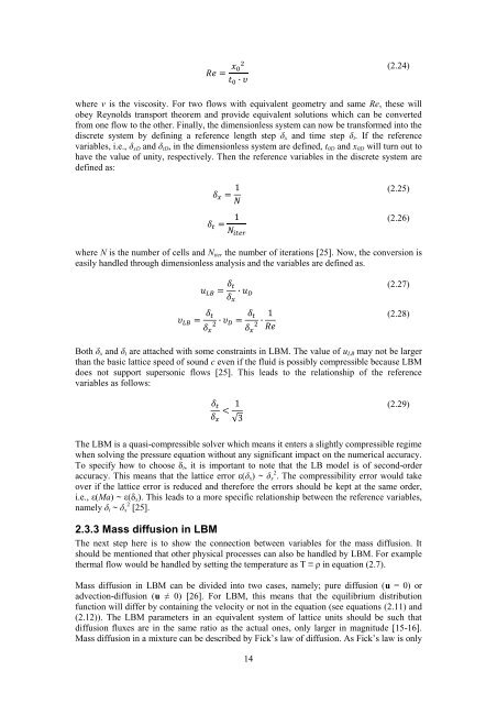
(2.24)<br />
where v is the viscosity. For two flows with equivalent geometry and same Re, these will<br />
obey Reynolds transport theorem and provide equivalent solutions which can be converted<br />
from one flow to the other. Finally, the dimensionless system can now be trans<strong>for</strong>med into the<br />
discrete system by defining a reference length step δ x and time step δ t . If the reference<br />
variables, i.e., δ xD and δ tD , in the dimensionless system are defined, t 0D and x 0D will turn out to<br />
have the value <strong>of</strong> unity, respectively. Then the reference variables in the discrete system are<br />
defined as:<br />
(2.25)<br />
(2.26)<br />
where N is the number <strong>of</strong> cells and N iter the number <strong>of</strong> iterations [25]. Now, the conversion is<br />
easily handled through dimensionless analysis and the variables are defined as.<br />
(2.27)<br />
(2.28)<br />
Both δ x and δ t are attached with some constraints in LBM. The value <strong>of</strong> u LB may not be larger<br />
than the basic lattice speed <strong>of</strong> sound c even if the fluid is possibly compressible because LBM<br />
does not support supersonic flows [25]. This leads to the relationship <strong>of</strong> the reference<br />
variables as follows:<br />
(2.29)<br />
The LBM is a quasi-compressible solver which means it enters a slightly compressible regime<br />
when solving the pressure equation without any significant impact on the numerical accuracy.<br />
To specify how to choose δ t , it is important to note that the LB model is <strong>of</strong> second-order<br />
accuracy. This means that the lattice error ε(δ x ) ~ δ x 2 . The compressibility error would take<br />
over if the lattice error is reduced and there<strong>for</strong>e the errors should be kept at the same order,<br />
i.e., ε(Ma) ~ ε(δ x ). This leads to a more specific relationship between the reference variables,<br />
namely δ t ~ δ x 2 [25].<br />
2.3.3 Mass diffusion in LBM<br />
The next step here is to show the connection between variables <strong>for</strong> the mass diffusion. It<br />
should be mentioned that other physical processes can also be handled by LBM. For example<br />
thermal flow would be handled by setting the temperature as T ≡ ρ in equation (2.7).<br />
Mass diffusion in LBM can be divided into two cases, namely; pure diffusion (u = 0) or<br />
advection-diffusion (u ≠ 0) [26]. For LBM, this means that the equilibrium distribution<br />
function will differ by containing the velocity or not in the equation (see equations (2.11) and<br />
(2.12)). The LBM parameters in an equivalent system <strong>of</strong> lattice units should be such that<br />
diffusion fluxes are in the same ratio as the actual ones, only larger in magnitude [15-16].<br />
Mass diffusion in a mixture can be described by Fick’s law <strong>of</strong> diffusion. As Fick’s law is only<br />
14