Probability and Statistics for Final Year Engineering Students

Point Estimation:
Probability and Statistics
for Final Year Engineering Students
By Yoni Nazarathy, Last Updated: May 24, 2011.
Exercises and Tutorial 3:
The Basics of Statistical Inference:
Point Estimation, Confidence Intervals and Hypothesis Testing
An estimator for some parameter of the population is said to be unbiased if = . For example,
the sample mean is an unbiased estimator for the population mean, the sample proportion is an
unbiased estimator for the sample proportion, but
∑
=
.
The estimator is said to be consistent if lim → = . Note: In this course we really didn’t define a
limit of random variables, yet in case of an unbiased estimator it is consistent if lim → = 0.
1. Consider the uniform distribution on the interval [a,b]. Let = , . Here are two estimators
for . (Note that here is a 2 dimensional vector).
I. = , .
II. A method of moments estimator which works as follows: We know the mean of the
distribution is =
. We know the variance is =
. We can estimate the
mean and variance using the standard estimators we have and then solve (for a and b):
=
and =
. This system is solved by = − √3 , = + √3 .
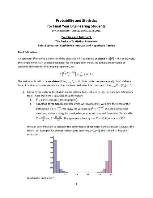
One can use simulation to compare the performance of estimator I and estimator II. Discuss the
results. For example, for 20 observations (and assuming a=0,b=1), this is the distribution of
estimator I:
Is estimator I unbiased?
1

As opposed to that, this is the distribution of estimator 2:
With 100 observations, this is the distribution of estimator I:
And this is the distribution of estimator II:
Which of the estimators is better? (There is not a “correct” answer to this).
2. Consider independent “noise” observations , , … which are assumed to have zero-mean
([ ]=0). Which of the following estimators are unbiased estimators for the variance?
(a) = ∑
(b) ∑
(c) ∑
2

Confidence Intervals:
A confidence interval for the population proportion is summarized as follows:
̂1 − ̂
̂ −
√
≤ ≤ ̂ +
̂1 − ̂
= 1 − .
√
Where is the x’th percentile (also called quantile) of the standard normal
distribution:
√
= . Here are typical values:
. = 1.645, . = 1.96, . = 2.576, . = 3.291.
The above statement is approximate due to two reasons:
1) The CLT is used.
2) p(1-p) is replaced by ̂1 − ̂.
When planning sample size
s, one can use the following formula (based on p(1-p)=1/4):
∗ =
4
.
3. An election poll between two candidates shows that 54% of the public supports candidate A. If
the number of questioned people is n=1000, write the following confidence intervals:
I. A 90% confidence interval.
II. A 95% confidence interval.
III. A 99% confidence interval.
IV. A 99.9% confidence interval.
4. We are planning an experiment for testing the proportion of bolts that can withstand a certain
load. We want to have an error of no more than 0.02 and be 99% percent confident. How many
bolts are needed?
5. The confidence interval formula presented above relies on the CLT (approximates the Binomial
distribution with the Normal distribution). In cases where n is not large and/or p is very close to
0 or 1, the normal approximation may be too crude. In this case, one can use the exact Binomial
distribution.
I. Discuss how to used the Binomial distribution instead of the normal (i.e. look at the
derivation of the confidence interval, what would you do differently)?
3

II. Why is using the Normal distribution computationally easier?
6. We did not explicitly discuss how to calculate a confidence interval for the population mean in
this course (only the proportions). Yet the concepts are the same. Assume that you are reading a
report by an external consultant which contains the following lines:
“… Randomly sampling 143 observations we have the following 95% confidence interval for the
population mean: 12.3 ± 1.1.”
Which of the following statements is True:
I. The sample mean was 12.3.
II. It is certain that the population mean is in the range [11.2, 13.4].
III. There is a 1 in 20 chance that the actual population mean is not in the range [11.2, 13.4]
IV. Should the study have had a confidence level of 99% instead of 95% the confidence
interval would have been wider.
4

Selected Solutions:
2)
a) Unbiased as shown in the lecture. This is the sample variance estimator.
b) ∑
=
=
so biased.
c) ∑
= [∑ ] = ∑ [
] =
[ ] =
(For a RV with zero mean, the variance is the expectation of X^2).
3) ̂ = 0.54.
I) 0.54±0.0259 II) 0.54±0.031 III) 0.54±0.041 IV) 0.54±0.052
4) 4148
6) I) True, II) False III)True IV) True.
5