The power of goodness of fit tests for close ... - ResearchGate

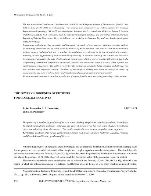
Measurement Techniques, Vol. 50, No. 2, 2007
The 4th International Seminar on “Mathematical, Statistical and Computer Support of Measurement Quality” was
held on June 28–30, 2006 in St Petersburg. The seminar was organized by the Federal Agency for Technical
Regulation and Metrology, COOMET, the Metrological Academy, the D. I. Mendeleev All-Russia Research Institute
of Metrology, and the PTB. Specialists from the national metrological institutes and universities of Russia, Ukraine,
Republic of Belarus, Kazakhstan, Kirgiz, Uzbekistan, Latvia, Bulgaria, Germany, England, and Sweden participated
in the proceedings.
Papers on methods of analyzing, processing and interpreting the results of measurements, including statistical methods
of estimating parameters and of taking decision, methods of Bayes statistics, and variance and multidimensional
analysis aroused traditional interest. A number of contributions were devoted to the use of statistical (computer)
modeling for solving problems of measurement data processing. A separate section of the seminar was devoted to
the problem of processing the data of international comparisons, which is now of considerable interest due to the
completion of international comparisons of national standards and the need to evaluate the data of key regional and
supplementary comparisons. The subjects covered by the seminar are constantly being expanded, and this year two
new sections were organized, namely, “Problems of metrological tracking used when processing the results of
measurements, and ways of solving them” and “Mathematical backup of analytical measurements.”
We draw readers’ attention to the following selection of papers from the most interesting proceedings of the seminar.
THE POWER OF GOODNESS OF FIT TESTS
FOR CLOSE ALTERNATIVES
B. Yu. Lemeshko, S. B. Lemeshko,
and S. N. Postovalov
UDC 519.24
The power of a number of goodness of fit tests when checking simple and complex hypotheses is analyzed
by statistical modeling methods. Estimates are given of the power of the tests when checking hypotheses
of certain relatively close alternatives. The results enable the tests to be arranged in order of power.
Key words: goodness of fit power, Kolmogorov, Cramer–von Mises–Smirnov, Anderson–Darling, Pearson,
and Rao–Robson–Nikulin, goodness of fit tests.
When using goodness of fit tests to check hypotheses that an empirical distribution, constructed from a sample taken
from a general set, corresponds to a theoretical law, simple and complex hypotheses can be distinguished. The simple hypothesis
under examination has the form H 0 : F(x) = F(x, θ), where F(x, θ) is the probability distribution function from which one
can check the goodness of fit of the observed sample and θ is the known value of the parameter (scalar or vector).
The complex hypothesis under examination can be written in the form H 0 : F(x) ∈ {F(x, θ), θ∈Θ}, where Θ is the
region in which the unknown parameter θ is defined. A difference arises in the use of tests when checking complex hypothe-
Novosibirsk State Technical University; e-mail: headrd@fpm.ami.nstu.ru. Translated from Izmeritel’naya Tekhnika,
No. 2, pp. 23–28, February, 2007. Original article submitted November 7, 2006.
132
0543-1972/07/5002-0132 © 2007 Springer Science+Business Media, Inc.

ses and corresponding problems if the estimate of the parameter q of a theoretical distribution is calculated using the same
sample with which the goodness of fit is verified. We will further assume that when checking complex hypotheses the estimate
of the parameter q is calculated using the same sample.
Two forms of error arise from the checked statistical hypotheses: errors of the 1st kind consists of the fact that, as a
result of checking, the true hypothesis H 0 deviates, while an error of the 2nd kind consists of recognizing the true hypothesis
H 0 when a certain competing hypothesis H 1 is correct.
The procedure for checking the hypothesis H 0 assumes that the distribution G(S⏐H 0 ) of the statistics S of the test
employed is known when H 0 is correct. For goodness of fit tests, the critical regions are characterized by large values of the
statistics. The probability α of an error of the 1st kind (the level of significance) is the probability that the value of the statistics
will fall in the critical region α = P{S > S α ⏐H 0 } = 1 – G(S α ⏐H 0 ), where S α is the critical value. As a rule, the value of
α is given when checking hypotheses. If the value of the statistics calculated from the sample S * ≤ S α ,one does not deviate
from the hypothesis H 0 under examination. A knowledge of the distribution G(S⏐H 0 ) enables one, from the value of S * ,to
obtain P{S > S * ⏐H 0 } = 1 – G(S * ⏐H 0 ) – the level of significance reached. One does not deviate from the hypothesis H 0 under
examination when P{S > S * ⏐H 0 } > α.
If a competing hypothesis H 1 is specified, we define the probability of an error of the 2nd kind by the relation β =
= P{S ≤ S α ⏐H 1 } = G(S α ⏐H 1 ), where G(S⏐H 1 ) is the distribution of the test statistics when H 1 holds. If the test is completely
defined, the specification of α uniquely defines the value of β and conversely. The power of a test 1 – β when checking the
hypothesis H 0 against H 1 is a function which depends on H 0 , H 1 , the volume of the sample n and, possibly, on certain other
factors, connected with the construction of the test.
When carrying out a statistical analysis of data, giving preference to a certain test, the experimentor wishes to have
assurance that, for a certain probability of an error α of the 1st kind, one is guaranteed a minimum probability of an error β of
the 2nd kind, i.e., one can choose the test which is the most powerful of the pair of alternatives H 0 and H 1 of interest to him.
The information in various sources regarding the advantages in certain situations of one goodness of fit test or another
is not unique, often contradictory, and subjective. Investigations of the power are made difficult by the lack of results connected
with the analytical representation of the distribution functions G(S⏐H 1 ) for specific goodness of fit tests when checking
complex hypotheses, in particular, for nonparametric tests and for χ 2 -type teests when estimating parameters from point
samples (from ungrouped observations).
The purpose of these investigations is to carry out a comparative analysis of the power of the goodness of fit tests
most often used on certain pairs of fairly close competing hypotheses H 0 and H 1 .
In the Kolmogorov test [1] statistics with a correction, proposed in [2], of the form
are most often used, where
6nDn
+ 1
Sk
= ,
6 n
+ − +
−
Dn = max( Dn , Dn ); Dn
= max{ i/ n− F( xi, θ)}; Dn
= max{ F( xi, θ) −( i−1) / n};
1≤≤
i n
1≤≤
i n
n is the volume of the sample; and x 1 , x 2 ,…,x n are sample values in increasing order. For the simple hypothesis under examination
to be correct, the statistics S k in the limit must obey the Kolmogorov distribution law K(s) [1].
The Cramer–von Mises–Smirnov ω 2 test statistics have the form [1]:
n
2
2 1 ⎧⎪
2i
− 1⎫⎪
Sω = nωn
= + ⎨Fxi
θ − ⎬
n
∑ ( , ) .
12
n
i=
1 ⎩⎪ 2 ⎭
When the simple hypothesis holds, the statistics in the limit must obey a law with the distribution function a1(s) [1].
133

The Anderson–Darling Ω test statistics is given by the expression [1]
n
⎧⎪
i −
⎛ i − ⎞
⎫
2
2 1
2 1
⎪
SΩ
= nΩ n = −n−2∑
⎨ ln Fx ( i, θ) + −
Fxi
n
⎜1
⎝ n
⎟ ln ( 1 − ( , θ)) ⎬,
⎠
i=
1 ⎩⎪ 2
2
⎭⎪
and when the simple hypothesis holds in the limit it must obey a law with distribution function a2(s) [1].
When checking simple hypotheses, the limit distributions of the statistics of these nonparametric tests are independent
of the form of the distribution law observed. They are therefore said to be distribution-free.
When checking complex hypotheses, when the parameters of the law are estimated from the same sample, nonparametric
tests lose the “distribution-free” property [3]. Moreover, the distributions of the test statistics become dependent
on the form of the complex hypothesis under examination [4].
The analytical form of the (limit) distributions of the statistics G(S⏐H 0 ) of nonparametric tests when checking complex
hypotheses is unknown. There are particular solutions in which different approaches are employed. Obviously, the most
promising one for constructing the distributions of the statistics is a numerical approach, based on statistical modeling of
empirical distributions of the statistics and the construction for them of approximate analytical models [4–8].
The use of the Pearson χ 2 test requires the region in which the random quantity is defined to be split into k intervals
and the calculation of the number of observations n i which fall within them, and the probabilities of them falling in the interval
P i (θ) corresponding to the theoretical law. The statistics of the test have the form
2
Xn
k
2
ni
n−
Pi
= n∑ ( / ( θ )) .
P
i=
1 i( θ)
(1)
When checking a simple valid hypothesis in the limit, the statistics obey a χ 2 k–1-distribution with k = 1 degrees of
freedom.
When checking a complex hypothesis when H 0 holds and under conditions that the estimates of the parameters are
2
found as a result of minimizing the statistics (1) using the same sample, the statistics X n is asymptotically distributed as
χ 2 k–r–1 ,where r is the number of parameters estimated from the sample. The statistics (1) have the same distribution if we
choose the maximum-likelihood method as the method of estimation and the estimates are calculated from classified data [9].
It has been shown by statistical modeling that this also occurs when using other asymptotically effective estimates based on
classified data [10].
When calculating maximum-likelihood estimates using unclassified data, the same statistics is subject to a law
which differs from the χk–r–1 2 -distribution. In this case, when checking complex hypotheses and using the maximum likelihood
estimates based on unclassified observations of the distribution G(X n⏐H0 ), the statistics of the test depend considerably
2
on the method of classification [11].
When preparing methods of statistical modeling, investigations were carried out on the distribution laws of χ 2 -type
statistics in the case of simple and different complex hypotheses, when the hypothesis H 0 holds together with a competing
hypothesis H 1 ,for equiprobable and asymptotically optimum classification [12]. In the asymptotically optimum classification,
the losses in the Fisher information are minimized, connected with the classification, and the power of the Pearson χ 2 test is
maximized with respect to the nearest competing hypotheses.
When checking complex hypotheses employing χ 2 -type tests, the use of estimates based on unclassified (point) observations
has definite advantages, since these estimates have the best asymptotic properties compared with estimates based on classified
data. Tests based on the Rao–Robson–Nikulin statistics [13] belong to tests of this kind. It is noteworthy that the statistics
of these tests when H 0 holds in the limit obey a χ 2 k–1-distribution irrespective of the number of parameters of the law, estimated
by the maximum-likelihood method, while the power of the test, as a rule, is greater than the power of the Pearson χ 2 test.
In this case, the statistics proposed by Nikulin [14–16] were considered. The test specifies the estimation of the
unknown parameters of the distribution F(x, θ) by the maximum-likelihood method using unclassified data. In this case, the
134

vector of the probabilities of falling in the intervals P = (P 1 , ..., P k ) T is assumed to be given, and the boundary points of the
intervals are found from the relations
The proposed statistics have the form [14]:
where X n
2 are calculated from (1); the matrix
−1
xi( θ ) = F ( P1 + ... + Pi), i = 1, ( k −1).
2 2 1
Yn
= Xn
+ n − a T ( θ) Λ( θ) a( θ),
−1
k wθ
w
li
θ ji
Λ( θ) = J( θl, θj) −∑
,
p
i=
1 i
the elements and dimensions of which are determined by the estimated components of the vector of the parameters θ;
J( θl, θj)
=
∫
⎛ ∂f( x, θ) ∂f( x, θ)
⎞
⎜
⎝ ∂θl
∂θ
⎟
j ⎠
f( x, θ)
dx
are the elements of the information matrix based on unclassified data, the components of the vector a(θ) have the form
a θ = w n P w n P
l θ l1 1/ 1+ ... + θ l k k / k
and
∂x
w f x
l i i i( θ)
θ =− [ ( θ), θ]
+
∂θl
∂xi−1( θ) f[ xi−1( θ), θ]
.
∂θl
N
When estimating the values of the power of the tests in order to construct empirical distributions G n (S⏐H0 ) and
N
G n (S⏐H1 ) of the corresponding statistics S, it is most convenient to use statistical modeling methods. To do this, one models
samples of the statistics S 1 , S 2 , ..., S N of a fairly large volume N for specific volumes of samples n of the observed quantities,
modeled using laws corresponding to the hypothesis under examination H 0 and the competing hypothesis H 1 . Further,
as a rule, N = 10 6 while the index N in the notation of the corresponding empirical functions is omitted.
We will illustrate the results of a comparative analysis of the power of the goodness of fit tests by two pairs of alternatives.
The normal and logistical laws comprise the first pair: the hypothesis H 0 under examination corresponded to a normal
law with density
1
⎧
⎪ ( x − θ ) ⎫
1 2 ⎪
f( x) = exp ⎨−
⎬,
2
θ0
2π
⎩⎪ 2θ0
⎭⎪
while the competing hypothesis H 1 corresponded to a logistical law with density function
π ⎪ ( x )
f( x) = exp
⎧− ⎨
π − θ ⎫
1 ⎪
⎬
θ0
3 ⎩⎪ θ0
3 ⎭⎪
2
⎡ ⎧
⎪ ( x )
+ exp ⎨− π − ⎫
⎢
θ
⎤
1 ⎪
1
⎬⎥
⎢
⎥
⎣ ⎩⎪ θ0
3 ⎭⎪
⎦
and the parameters θ 0 = 1 and θ 1 = 0. In the case of the simple hypothesis H 0 , the parameters of the normal law have the
same values. Since these two laws are very close, it is difficult to distinguish them using goodness of fit tests.
135

TABLE 1. Power of the Goodness of Fit Tests When Checking a Simple Hypothesis H 0 (a normal
distribution) Against an Alternative H 1 (logistical)
Significance
Value of the power for n
level α 100 200 300 500 1000 2000
Pearson χ 2 test for k = 15 and asymptotically optimal classification
0.15 0.349 0.459 0.565 0.737 0.946 0.999
0.1 0.290 0.388 0.490 0.671 0.922 0.998
0.05 0.210 0.292 0.385 0.565 0.871 0.996
0.025 0.154 0.222 0.302 0.472 0.813 0.992
0.01 0.107 0.159 0.221 0.369 0.729 0.983
Anderson–Darling Ω 2 test
0.15 0.194 0.258 0.328 0.472 0.776 0.982
0.1 0.125 0.169 0.222 0.343 0.654 0.957
0.05 0.057 0.079 0.107 0.181 0.439 0.869
0.025 0.026 0.036 0.049 0.088 0.261 0.724
0.01 0.010 0.013 0.017 0.031 0.114 0.491
Kolmogorov test
0.15 0.190 0.246 0.303 0.415 0.662 0.922
0.1 0.127 0.170 0.215 0.309 0.544 0.861
0.05 0.062 0.088 0.116 0.179 0.365 0.721
0.025 0.031 0.044 0.061 0.100 0.231 0.560
0.01 0.012 0.018 0.026 0.044 0.119 0.366
Cramer–von Mises–Smirnov ω 2 test
0.15 0.178 0.228 0.283 0.401 0.680 0.947
0.1 0.114 0.147 0.186 0.277 0.542 0.892
0.05 0.052 0.067 0.086 0.136 0.324 0.742
0.025 0.024 0.030 0.039 0.062 0.171 0.548
0.01 0.010 0.011 0.014 0.021 0.065 0.307
The second pair was as follows: H 0 is a Weibull distribution with density
θ
θ0( x − θ1)
f( x)
=
θ0
θ1
−1
⎧
θ
⎛ ( x − ) ⎞
0 ⎫
⎪ θ2
⎪
exp ⎨−⎜
⎟ ⎬
⎪ ⎝ θ1
⎠
⎩
⎭
⎪
and parameters θ 0 = 2, θ 1 = 2, and θ 2 = 0; H 1 is a gamma distribution with density
0
θ
⎛ x − ⎞
0 −1
1 θ2
f( x)
=
exp[ ( x ) / ]
( )
⎜ ⎟ − −θ2 θ1
θ1Γ
θ0
⎝ θ1
⎠
and parameters θ 0 = 3.12154, θ 1 = 0.557706, and θ 2 = 0, for which the gamma distribution is closest to this Weibull distribution.
We investigated the power when checking simple and complex hypotheses H 0 against the simple alternative H 1 .
We used the maximum-likelihood method when checking complex hypotheses in the case of all the goodness of fit
tests investigated in order to estimate the unknown parameters. Here all the tests were under equal conditions. Moreover,
136

TABLE 2. Power of the Goodness of Fit Tests When Checking a Complex Hypothesis H 0 (a normal distribution) Against an
Alternative H 1 (logistical)
Significance
Value of the power for n
level α 20 50 100 200 300 500 1000 2000
Anderson–Darling Ω 2 test
0.15 0.222 0.297 0.400 0.575 0.708 0.873 0.989 1.000
0.1 0.164 0.230 0.324 0.496 0.636 0.828 0.981 1.000
0.05 0.098 0.149 0.224 0.377 0.519 0.741 0.963 1.000
0.025 0.060 0.096 0.152 0.282 0.414 0.649 0.935 0.999
0.01 0.031 0.054 0.091 0.186 0.297 0.525 0.885 0.998
2
Nikulin Y n test for k = 15 and asymptotically optimum classification
0.15 0.245 0.320 0.395 0.536 0.646 0.806 0.967 1.000
0.1 0.195 0.249 0.332 0.466 0.579 0.755 0.952 0.999
0.05 0.137 0.165 0.248 0.368 0.480 0.669 0.921 0.998
0.025 0.077 0.112 0.184 0.291 0.395 0.587 0.883 0.996
0.01 0.036 0.071 0.125 0.213 0.304 0.488 0.825 0.992
Cramer–von Mises–Smirnov ω 2 test
0.15 0.210 0.273 0.366 0.529 0.659 0.836 0.980 1.000
0.1 0.153 0.208 0.291 0.447 0.582 0.781 0.968 1.000
0.05 0.090 0.130 0.194 0.329 0.458 0.678 0.939 0.999
0.025 0.053 0.082 0.128 0.237 0.353 0.573 0.897 0.998
0.01 0.027 0.044 0.074 0.150 0.243 0.445 0.825 0.994
Pearson χ 2 test for k = 15 and asymptotically optimal classification
0.15 0.243 0.295 0.342 0.467 0.579 0.751 0.950 0.999
0.1 0.194 0.220 0.280 0.393 0.502 0.688 0.928 0.998
0.05 0.140 0.133 0.199 0.291 0.391 0.583 0.882 0.996
0.025 0.081 0.080 0.137 0.214 0.303 0.486 0.827 0.992
0.01 0.036 0.043 0.079 0.139 0.213 0.376 0.745 0.984
Kolmogorov test
0.15 0.200 0.246 0.313 0.440 0.554 0.732 0.941 0.999
0.1 0.142 0.181 0.236 0.351 0.459 0.646 0.905 0.997
0.05 0.080 0.105 0.143 0.230 0.322 0.502 0.823 0.990
0.025 0.045 0.061 0.086 0.149 0.219 0.376 0.721 0.975
0.01 0.021 0.029 0.043 0.081 0.127 0.244 0.575 0.938
TABLE 3. Power of the Test for Checking the Deviation of a Distribution from a Normal Law
Against an Alternative H 1 (a logistical law)
Significance
Value of the power of the test for n = 20 and 50
level Shapiro–Wilk Epps–Pally D’Agostino with z 2
α
20 50 20 50 20 50
0.1 0.181 0.202 0.178 0.249 0.189 0.327
0.05 0.117 0.141 0.111 0.165 0.111 0.223
0.01 0.044 0.067 0.037 0.062 0.032 0.089
137

TABLE 4. Power of the Goodness of Fit Tests for Checking a Simple Hypothesis H 0 (a Weibull
distribution) Against an Alternative H 1 (a gamma distribution)
Significance
Value of the power for n
level α 100 200 300 500 1000 2000
Pearson χ 2 test for k = 15 and the asymptotically optimum classification
0.15 0.486 0.621 0.757 0.909 0.996 1.000
0.1 0.418 0.556 0.701 0.876 0.993 1.000
0.05 0.324 0.469 0.611 0.815 0.986 1.000
0.025 0.254 0.403 0.529 0.751 0.974 1.000
0.01 0.191 0.332 0.437 0.668 0.954 1.000
Anderson–Darling Ω 2 test
0.15 0.302 0.446 0.577 0.781 0.976 1.000
0.1 0.223 0.348 0.473 0.689 0.951 1.000
0.05 0.131 0.224 0.326 0.533 0.882 0.998
0.025 0.076 0.141 0.220 0.396 0.785 0.993
0.01 0.037 0.075 0.126 0.257 0.636 0.975
Cramer–von Mises–Smirnov ω 2 test
0.15 0.295 0.425 0.539 0.716 0.931 0.998
0.1 0.224 0.343 0.453 0.637 0.894 0.995
0.05 0.138 0.233 0.329 0.508 0.816 0.987
0.025 0.084 0.155 0.233 0.393 0.725 0.970
0.01 0.043 0.088 0.142 0.270 0.597 0.934
Kolmogorov test
0.15 0.294 0.421 0.531 0.700 0.915 0.995
0.1 0.225 0.342 0.450 0.628 0.879 0.992
0.05 0.141 0.237 0.332 0.508 0.806 0.981
0.025 0.087 0.160 0.239 0.401 0.723 0.964
0.01 0.045 0.093 0.150 0.282 0.606 0.930
the Kolmogorov, Cramer–von Mises–Smirnov ω 2 , and Anderson–Darling Ω 2 type nonparametric tests are the most powerful
compared with the case when the estimates are found by minimizing the corresponding statistics [6].
In Table 1, we show estimates of the power of the goodness of fit tests considered, calculated from the results of
modeling distributions of the statistics, in the case of a pair of normal–logistical alternatives for different values of the significance
level α when checking a simple hypothesis H 0 , corresponding to a normal law with parameters (0, 1), against an
alternative H 1 , corresponding to a logistical law with the same set of parameters. The error of the estimates of the power
when checking the simple hypotheses and a 95% confidence interval does not exceed ±10 –3 . The tests are arranged in order
of decreasing power.
In Table 1, we show the maximum power of the Pearson χ 2 test, which it has for a given pair of alternatives for k =15
and asymptotically optimum classification. For equiprobable classification, the Pearson χ 2 test against a given pair of alternatives
has maximum power for k = 4 [17]. Further, the power falls off as k increases. But this maximum level of power is
less than the power of the given test when k = 9 and using the asymptotically optimum classification.
Estimates of the power when checking a complex hypothesis H 0 , corresponding to the observed sample having a
normal law against the same simple competing hypothesis H 1 ,are shown in Table 2. Here also the criteria are arranged in
order of decreasing power. It should be noted that in certain cases the preference is not obvious since, although possessing
138

TABLE 5. Power of the Goodness of Fit Tests When Checking a Complex Hypothesis H 0 (a Weibull
distribution) Against an Alternative H 1 (a gamma distribution)
Significance
Value of the power for n
level α 100 200 300 500 1000 2000
Anderson–Darling Ω 2 test
0.15 0.435 0.667 0.817 0.952 0.999 1.000
0.1 0.353 0.589 0.757 0.928 0.998 1.000
0.05 0.244 0.466 0.650 0.876 0.995 1.000
0.025 0.167 0.361 0.547 0.811 0.990 1.000
0.01 0.100 0.252 0.424 0.715 0.977 1.000
Cramer–von Mises–Smirnov ω 2 test
0.15 0.396 0.603 0.750 0.913 0.996 1.000
0.1 0.316 0.520 0.679 0.875 0.993 1.000
0.05 0.212 0.394 0.560 0.797 0.984 1.000
0.025 0.143 0.295 0.452 0.712 0.968 1.000
0.01 0.082 0.196 0.330 0.593 0.936 1.000
Nikulin Y 2 n test for k = 9 and asymptotically optimum classification
0.15 0.324 0.511 0.665 0.869 0.993 1.000
0.1 0.246 0.423 0.584 0.818 0.987 1.000
0.05 0.153 0.299 0.454 0.720 0.973 1.000
0.025 0.096 0.209 0.347 0.619 0.951 1.000
0.01 0.051 0.129 0.238 0.492 0.909 0.999
Pearson χ 2 test for k = 9 and asymptotically optimum classification
0.15 0.347 0.525 0.678 0.868 0.992 1.000
0.1 0.273 0.439 0.596 0.818 0.986 1.000
0.05 0.172 0.311 0.463 0.719 0.970 1.000
0.025 0.104 0.218 0.352 0.617 0.946 1.000
0.01 0.053 0.133 0.237 0.483 0.898 0.999
Kolmogorov test
0.15 0.340 0.510 0.646 0.830 0.981 1.000
0.1 0.262 0.420 0.558 0.762 0.965 1.000
0.05 0.164 0.293 0.420 0.640 0.925 0.999
0.025 0.101 0.200 0.306 0.519 0.867 0.997
0.01 0.052 0.115 0.193 0.375 0.763 0.988
a higher power for some levels of significance and some sample volumes, the test may lose out for other values of α and n.
In Table 2, the maximum power of the Nikulin and Pearson χ 2 tests is shown.
When estimating the power when checking complex hypotheses, we based ourselves on modeled distributions of the
statistics G(S⏐H 0 ) for a sample volume n = 1000. With such large values of n, the empirical distribution of the statistics can
be assumed to be a good estimate of the limit law.
When checking complex hypotheses and sample volumes n = 20 and 50 for all the tests investigated, the distributions
G(S 20 ⏐H 0 ) and G(S 50 ⏐H 0 ) differ considerably from the “limit” distribution G(S n ⏐H 0 ) for n = 1000. Hence the power
was estimated from modeled pairs of distributions of the form G(S 20 ⏐H 0 ), G(S 20 ⏐H 1 ) and G(S 50 ⏐H 0 ), G(S 50 ⏐H 1 ).
139

The power of the goodness of fit tests for small sample volumes n can be compared with the power of tests constructed
specially to check the deviation of a distribution from a normal law: using the Shapiro–Wilk, Epps–Pally, and
D’Agostino tests with statistics z 2 . Estimates of the power of these tests of normality, obtained in [18] and improved in the
present paper for volumes of the modeled samples of the statistics N = 10 6 ,are shown in Table 3, from which it follows that
the “special” tests against the pair of alternatives considered turn out to be of somewhat greater power on average.
The calculated estimates of the power of the tests for different values of the level of significance α when checking
the goodness of fit with the Weibull distribution (hypothesis H 0 ) against an alternative, corresponding to the gamma-distribution
with these parameters (hypothesis H 1 ) for the simple hypothesis H 0 are shown in Table 4, and a complex hypothesis
H 0 in Table 5. The tests in these tables are listed in order of decreasing power.
Hence, for the case when checking simple hypotheses, the tests can be listed in order of power as follows:
Pearson (asymptotically optimum classification) χ 2 P Anderson–Darling Ω 2 P von Mises ω 2 P= Kolmogorov.
This scale holds when using the Pearson (asymptotically optimal classification) χ 2 in the test, for which the losses
in Fisher information are minimized. For very close hypotheses, we may have
Kolmogorov P von Mises ω 2 .
When checking complex hypotheses, the power gradation turns out to be quite different:
Anderson–Darling Ω 2 P von Mises ω 2 P Y n
2 (asymptotically optimum classification) P
P Pearson (asymptotically optimum classification) X n
2 P Kolmogorov.
For very close hypotheses, we may have
Anderson–Darling Ω 2 P Y n
2 (asymptotically optimum classification) P von Mises ω
2 P
P Pearson (asymptotically optimum classification) χ 2 P Kolmogorov.
These conclusions have an integrated form. The ordering is not rigid. As can be seen from the tables with listed
values of the power, sometimes a test has advantages in power for some values of α and sample volumes n but is inferior for
other values of α and n.
It should be borne in mind that the power of the Pearson and Nikulin χ 2 type tests depends not only on the hypotheses
H 0 and H 1 and the sample volume n,but, for specified H 0 and H 1 , on the method of classification and the number of intervals.
The number of intervals for which the power of the tests for a pair of alternatives H 0 and H 1 is a maximum depends on
these hypotheses and on the method of classification. An increase in the number of intervals does not always lead to an
increase in the power of χ 2 type tests [17].
For close hypotheses H 0 and H 1 , the choice of asymptotically optimum classifications when using the Pearson χ 2
test gives a positive effect for simple and complex hypotheses. However, this does not mean that the use of asymptotically
optimum classifications always guarantees maximum power of the test. For specific and not very close hypotheses, certain
other methods of classification may turn out to be optimum, which can be obtained as a result of maximizing the test power.
For one and the same pair of hypotheses H 0 and H 1 for one number of intervals k, the Nikulin test may turn out to
have a greater power with the asymptotically optimum classification, while for a different k it may be more powerful for an
equiprobable classification. The dependence of the power of a given test on the method of classification turns out to be more
complex and requires further investigation.
This research was supported by the Ministry of Education and Science of the Russian Federation (project No. 2006-
RI-19.0/001/119) and the Russian Fund for Basic Research (project No. 06-01-00059-a).
140

REFERENCES
1. L. N. Bol’shev and N. V. Smirnov, Tables of Mathematical Statistics [in Russian], Nauka, Moscow (1983).
2. L. N. Bol’shev, Teor. Veroyat. Primenen., 8, No. 2, 129 (1963).
3. M. Kac, J. Kiefer, and J. Wolfowitz, Ann. Math. Stat., 26, 189 (1955).
4. R 50.1.037-2002, Recommendations on Standardization. Applied Statistics. Rules for Checking the Goodness of Fit
of an Experimental Distribution with Theoretical Ones. Pt. II. Nonparametric Test [in Russian], Izd. Standartov,
Moscow (2002).
5. B. Yu. Lemeshko and S. N. Postovalov, Zavod. Lab., 64, No. 3, 61 (1998).
6. B. Yu. Lemeshko and S. N. Postovalov, Zavod. Lab., 67, No. 7, 62 (2001).
7. B. Yu. Lemeshko and S. N. Postovalov, Avtometr., No. 2, 88 (2001).
8. B. Yu. Lemeshko and A. A. Maklakov, Avtometr., No. 3, 3 (2004).
9. G. Cramer, Mathematical Methods of Statistics [Russian translation], Mir, Moscow (1975).
10. B. Yu. Lemeshko and E. V. Chimitova, Zavod. Lab. Diagnostika, Materialov, 70, No. 1, 54 (2004).
11. R 50.1.033-2001, Recommendations on Standardization. Applied Statistics. Rules for Checking the Goodness of Fit
of an Experimental Distribution with Theoretical Ones. Pt. I. Chi-Squared Type Tests [in Russian], Izd. Standartov,
Moscow (2002).
12. B. Yu. Lemeshko, Zavod. Lab., 64, No. 1, 56 (1998).
13. A. W. Van der Vaart, Asymptotic Statistics, University Press, Cambridge (1998).
14. M. S. Nikulin, Teor. Veroyat. Primeneniya, XVIII, No. 3, 675 (1973).
15. M. Mirvaliev and M. S. Nikulin, Zavod. Lab., 58 No. 3, 52 (1992).
16. P. E. Greenwood and M. S. Nikulin, A Guide to Chi-Squared Testing, John Wiley, New York (1996).
17. B. Yu. Lemeshko and E. V. Chimitova, Zavod. Lab. Diagnostika Materialov, 69, No. 1, 61 (2003).
18. B. Yu. Lemeshko and S. B. Lemeshko, Metrologiya, No. 2, 3 (2005).
141