STABILITY AND CHAOS IN PASSIVE-DYNAMIC ... - Cornell University

STABILITY AND CHAOS IN PASSIVE-DYNAMIC LOCOMOTION 

M.J. COLEMAN, M. GARCIA, A. L. RUINA AND J. S. CAMP 

Department of Theoretical and Applied Mechanics 

Cornell University, Ithaca, NY 14853-7501 

AND 

A. CHATTERJEE 

Engineering Science and Mechanics 

Penn State University, University Park, PA 16802 

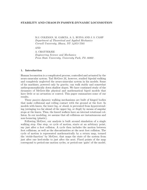
1. Introduction 

Human locomotion is a complicated process, controlled and actuated by the 

neuro-muscular system. Tad McGeer [8], however, studied bipedal walking 

and completely neglected the neuro-muscular system in his models. Some 

of his machines, powered only by gravity, can walk stably and somewhat 

anthropomorphically down shallow slopes. We have continued study of the 

dynamics of McGeer-like physical and mathematical biped models that 

have little or no actuation or control. This paper summarizes some of our 

results. 

These passive-dynamic walking mechanisms are built of hinged bodies 

that make collisional and rolling contact with the ground at the foot. In 

models with knees, the lower leg, or shank, is prevented from hyperextending 

(swinging too far ahead of the upper leg, or thigh) by means of angular 

stops at the knees. Thus, the kneed walkers have an internal rotational collision. 

In our modeling, we assume that all collisions are instantaneous and 

non-bouncing (plastic). 

Following McGeer, our analysis is built around simulation of a single 

walking step. One step, or cycle of motion, starts at an arbitrary point, 

say just after a foot collision. A cycle then includes the motion between 

foot collisions, as well as the discontinuities at the next foot collision. The 

cycle of motion is represented mathematically by a return map, termed 

the ‘stride-function’ by McGeer, that maps the state of the system from 

just after one heel-strike to just after the next. Fixed points of the map 

correspond to period-one motion cycles, or period-one ‘gaits’ of the model.

2 M.J. COLEMAN ET AL. 

Gait stability can be determined by calculating (most often numerically) 

the eigenvalues of the linearization of the map at the fixed points (see [3] 

for a detailed description of the modeling and analysis procedures). 

(a) 

x 

κ 

G 

r 

z 

D 

crooked 

masses; I G , m C 

disc; I D , m D 

massless fork 

y 

L 

E 

(b) 

downslope 

plane of 

wheel 

l 

m, I C 

C 

x F 

fixed coord. 

syst. α 

n = number of 

spokes 

g 

β = 2π n 

rest 

configuration 

z F 

y F 

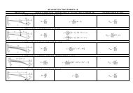
Figure 1. The parameters and orientation variables for (a) a uniform rolling disk with 

oblique masses added and (b) a rimless spoked wheel. 

Using this scheme, we have studied several passive-dynamic models of 

increasing complexity, progressing from rolling wheels to 2D straight-legged 

and kneed models to 3D straight-legged models, each of which is described 

below. We also describe a simple barely-controlled powering scheme for a 

2D straight-leg walker, which produces stable gait on level ground. 

2. Rolling Wheels in 2D and 3D 

Perhaps the simplest passive-dynamic system to study, that has some features 

in common with walking, is the rimless spoked wheel, or rolling polygon, 

confined to 2D [8]. The 2D rimless wheel has a stable limit cycle motion 

whose eigenvalues and associated global basins of attraction we have completely 

determined analytically [3]. The primary lesson of the rimless wheel 

in 2D is that speed regulation comes from a balance of collisional dissipation, 

which is proportional to speed squared, and gravitational work, which 

is proportional to speed. 

Next, we studied a 3D rolling disk with oblique masses added [3] (see 

Figure 1). The masses can bank and steer with the disk but cannot roll (or 

pitch) with it. The purpose of this investigation was to study the effects 

of mass distribution on stability. The oblique masses, if adjusted properly, 

change the stability of the uniform rolling disk, a conservative nonholonomic 

system, from neutrally stable to asymptotically stable [10]. This result 

suggests that mass distribution may affect side-to-side balance in more 

complicated walking models. 

Finally, we studied the 3D rimless wheel (see Figure 1) and found analytically, 

for many spokes and small slope angles, the stability eigenvalues 

for steady ‘rolling’ motions [1]. The 3D rimless wheel is a piecewise-

STABILITY AND CHAOS IN PASSIVE-DYNAMIC LOCOMOTION 3 

conservative-holonomic (but globally non-conservative and nonholonomic) 

system with intermittent, dissipative impacts – features that are shared by 

some more realistic human walking models. The rolling rimless wheel can 

also exhibit asymptotic stability when perturbed from a downhill limit cycle, 

even when its mass distribution corresponds to that of a disk that does 

not have asymptotic stability. Thus, the intermittent collisions can play a 

role in side-to-side balance. 

Despite the useful lessons from rolling models, they are not anthropomorphic 

walkers. They cannot fall down forwards or backwards, and they 

lack swinging legs. 

3. Straight-Legged 2D Walkers 

The next-simplest class of models live in 2D and consist of two linked swinging 

legs and point-feet [8, 6, 3, 5]. Asymptotically-stable walking motions 

of these models exist for a variety of parameters. The simplest such ‘pointfoot’ 

straight-legged model has a huge hip mass and tiny masses (relatively 

infinitesimal) at its point-feet (see Figure 2). 

A typical plot of the stance-leg and swing-leg angles is shown over one 

stable step in Figure 2. This model exhibits two steady walking motions, 

or period-one gaits, all the way to γ → 0 + as shown in Figure 3. At these 

gaits, the stance angle (and step length) are proportional to γ 1/3 . Figure 4 

shows how stable limping (period-two) and apparently-chaotic ‘staggering’ 

gaits appear as the slope angle is increased. 

That this machine can walk on arbitrarily small slopes means that, 

by some reasonable measures, it is capable of near-perfectly-efficient gait 

(zero+ energy cost per unit distance of transport). At small slopes, the 

gravitational power used by this model in downhill walking is proportional 

to the fourth power of the walking speed. This result gives insight into 

achieving similar efficiency in more complicated models (e.g. models with 

knees, circular feet, and/or more general mass distribution). The power 

scaling depends, in part, on the infinitesimally small feet. With finite-mass 

feet, there are two modes of energy loss at heelstrike: one due to deflection 

of the hip mass, and one due to dissipation of the foot’s kinetic energy in a 

plastic collision with the ground. Preliminary studies of point-foot models 

with finite foot mass show that the long-period gaits retain the same scaling 

laws at small slopes, while the short-period gaits do not. 

4. More General 2D Walkers 

We have reproduced and extended McGeer’s results for more general 2D 

walkers with knees[8]: Figure 5 shows the state variables and parameters for


0.25 

0.2 

swing leg angle θ sw 

γ = 0.009 rad 

m


negative stance angle at fixed point, -θ ∗ st , rad 

0.3 

0.25 

0.2 

0.15 

0.1 

0.05 

long period 

solutions 

stable gait solutions, 

analytic and numerical 

(heavy line) 

stable higher-period 

solutions (see inset) 

stable walking down to zero slope 

short period 

solutions (always unstable) 

analytic approx. 

numerical points 

0 

0 0.005 0.01 0.015 0.02 0.025 0.03 0.035 0.04 0.045 

slope γ, rad 

x 

Figure 3. Comparison of numerical and analytic predictions for point-foot stance angle 

at fixed point as a function of slope. The box is shown expanded in Figure 4. 

negative stance angleat fixed point -θ ∗ st, rad 

0.27 

0.26 

0.25 

0.24 

stable period-2 gait 

stable 

period-1 

gait 

stable period-4 gait 

unstable 

period-1 gaits 

didn't find stable solutions here 

0.014 0.015 0.016 0.017 0.018 0.019 0.02 

slope γ , rad 

'normal' gait limping gait 4,8,...-step & 'chaos' 

Figure 4. Period doubling of stable walking motions, inset from Figure 3. Period doubling 

occurs when one of the map eigenvalues for a period-n walking cycle passes through −1. 

Unstable period-one cycles are shown for reference. Dotted lines represent stable cycles 

while solid lines represent unstable ones. No persistent walking was found at slopes much 

steeper than 0.019 radians. 

legged Tinkertoy R○ model that walks passively, apparently stably, down 

gentle slopes [2] (see Figure 7).


a) DIMENSIONAL PARAMETERS 

b) DYNAMIC VARIABLES 

r T 

, m T 

r S 

, m S 

l T cT 

g 

w S 

ε T 

R 

ε T 

w T 

c S 

ε T 

θsh 

θth 

-θst 

γ 

l S 

ε T 

Figure 5. McGeer’s kneed walking model. Shown above are (a) model parameters, and 

(b) dynamic variables. Radii of gyration and masses of thigh and shank are denoted by 

r T ,m T,r S, and m S, respectively. The foot is a circular arc centered at the “+”. ɛ T is 

defined to be the angle between the stance thigh and the line connecting the hip to the 

foot center. Dynamic variable values θ st, θ th , and θ sh are measured from ground-normal 

to lines offset by ɛ T from their respective segments. A stop (not shown) at each knee 

prevents hyperextension of either knee. 

The configuration and mass distribution of the legs of the Tinkertoy R○ 

model were suggested by numerical simulations of a simpler 3D model (see 

Figure 8) that was predicted to be almost-stable. The model predicts nearstable 

steady 3D walking solutions (the maximum return map eigenvalue 

is |σ| max ≈ 1.15 with all others σ ≤ 1) for very low center-of-mass and 

lateral center-of-mass location comparable to the leg length. As the lateral 

center-of-mass position get very large, the model predicts something like 

‘tight-rope’ walking with a long balance bar: the step period and length get 

very small, and the maximum map eigenvalue modulus approaches 1 (neutral 

stability) asymptotically from above (see Figure 10). More detailed 3D 

modeling is currently in progress. This walking mechanism joins a small 

list of passive mechanical devices free to move in three dimensions but 

without fast spinning parts, that are statically unstable, yet can be dynamically, 

asymptotically stable. Figure 9 shows typical 3D periodic behavior 

predicted by the model. 

6. Powered ‘Passive’ Walking 

Once power is added to our passive devices, they are, of course, no longer 

uncontrolled in the pure sense. Nevertheless, as shown by McGeer [7], a 

stable passive-dynamic model is a good basis for simple ‘open-loop’ powering 

schemes. Figure 11 shows the configuration and simulated walking 

cycle for a powered 2D point-foot-like model. The torque is provided by a 

constant-voltage DC motor at the stance-ankle. The ankle is locked during 

the passive mode.


leg angles (rad) 

0.5 

0.4 

0.3 

0.2 

0.1 

0 

-0.1 

-0.2 

-0.3 

-0.4 

-0.5 

θ sh 

θ th 

heelstrike 

heelstrike 

θ st 

kneestrike 

θ sh =θ th 

3 3.5 4 4.5 5 5.5 

time, [(l S +l T )/g ] 1/2 

3 link mode 2 link mode 

1 step 

Heelstrike 3 Link Mode Kneestrike 2 Link Mode Heelstrike 

Simulated single-leg strobe-shots Human data including trunk (from 

(A little more than two steps) Winter 1987, used with permission) 

γ=0.036 

.2 m 

.2 m 

Figure 6. Simulated gait cycle (ours, similar to McGeer’s). Angles of leg segments are 

shown from just before one heelstrike to just after the next heelstrike in a stable gait of 

the walker in Figure 5. The heavy line on the graph corresponds to the motion of the 

heavy-line leg on the small cartoon under the graph. At the start of the step, this is the 

stance leg, but it becomes the swing leg just after the first heelstrike. The strobe-like 

picture of the walker on the bottom left, created from the simulated gait cycle in the 

graph, shows the anthropomorphic nature of the gait. The stroboscopic picture on the 

lower right was generated from experimental data from [11]. The parameters values used, 

from a working physical model in our lab, are: l t =0.35m, w t = 0m, m t =2.345kg, 

r t =0.099m, c t =0.091m, l s =0.46m, w s =0.025m, m s =1.013kg, r s =0.197m, 

c s =0.17m, R =0.2m, γ =0.036rad, g =9.81 m/s 2 , ɛ T =0.097rad. 

7. Conclusions 

The human-like and complicated motions of McGeer-like passive dynamic 

devices studied by ourselves and others imply that coordination in locomotion 

may be largely governed by pure mechanics. It has yet to be determined 

whether or not these models have medically-useful lessons to teach us, and 

whether or not they are a good spring-board for biomechanical or robotic


metal nuts 

brass strips 

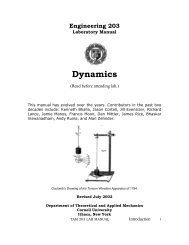
Figure 7. A drawing of our 3D Tinkertoy R○ walking model. The center-of-mass of the 

device is above the centers of the wheel-like feet and behind the leg axes. The metal 

nuts for weight and the brass strips to round the foot bottoms are fastened with black 

electrical tape. 

a) Dimensional Parameters 

X cm 

sw 

hinge 

joint 

plane of walker 

Y st 

cm 

X sw 

cm 

ball-and-socket 

joint 

x SW 

z ST 

z SW 

y SW 

x ST 

Z st 

cm 

y ST 

Y sw 

cm 

z F 

y F 

x F 

α 

l 

Z sw 

cm 

downslope 

g 

rest 

configuration 

swing leg 

b) Orientation Variables 

z ST 

θ sw 

z SW 

θ st 

x ST 

ψ 

φ 

y SW 

ψ 

x SW 

rotated 

stance frame 

configuration 

θ st 

stance leg 

Figure 8. The orientation variables and parameters for the 3D straight-legged point-foot 

walking model. Each leg has mass M, moment of inertia matrix I cm , and length l. 

y ST 

models that incorporate neuro-muscular elements or mechanical actuators. 

References 

1. M. Coleman, A. Chatterjee, and A. Ruina. Motions of a rimless spoked wheel: A 

simple 3D system with impacts. Dynamics and Stability of Systems, 1997. In press. 

2. M. Coleman and A. Ruina. A Tinkertoy R○ model that walks. Physical Review 

Letters, 1997. accepted for publication. 

3. M. J. Coleman. A Stability Study of a Three-dimensional Passive-dynamic Model 

of Human Gait. PhD thesis, Cornell University, Ithaca, NY, 1997. In preparation. 

4. J. V. Fowble and A. D. Kuo. Stability and control of passive locomotion in 3-D.


(a) 0.1 


0.05 

0 

-0.05 

-0.1 

-0.15 

stance leg swing leg angle, 

angle, θ* st (τ) θ* 

sw (τ)+θ * st (τ)-π 

-0.2 

0 0.2 0.4 0.6 0.8 1 1.2 1.4 

τ, non-dimensional time 

(b) 2 x 10-3 1 bank 

0 

-1 

-2 

heading 

heading, φ and bank, ψ 

-3 

-4 

-5 

0 0.2 0.4 0.6 0.8 1 1.2 1.4 

τ, non-dimensional time 

Figure 9. Simple 3-D simulations. Typical periodic gait cycle behavior over two steps 

for I xx = 0.5577, I yy = 0.00021, I zz = 0.5579, I xy = 0.0000, I xz = 0.0, I yz = 0.0, 

α = 0.0037,x = 0.0, y = 0.2706, and z = 0.9270. The fixed point for this case is 

q ∗ = {0.0000 0.000008 − 0.0597 3.2610 − 0.0132 0.00051 0.1866 − 0.8523} T ; the maximum 

eigenvalue is |σ max| =2.58 and the non-dimensional step period is τ ∗ =1.2031. 

(a) The periodic gait cycle leg angles are very similar to those for 2D walking. The 

heavy line on the graph corresponds to the motion of the heavy-lined leg in Figure 8. 

At start-of-step, this is the stance leg, but at a foot-collision, it becomes the swing leg. 

The instants of foot-strike are denoted by the light gray lines. (b) The plots show the 

relationship of the heading and the bank angle of the walker over two steps. 

τ*, step period 

1.4 

1.2 

1 

0.8 

0.6 

0.4 

0 0.5 1 1.5 2 

lateral c.o.m. position 

* 

-0.04 

-0.05 

-0.06 

-0.07 

0 0.5 1 1.5 2 


θst , stance angle-0.03 

|σ| max , max. eigenvalue 

3 

2.5 

2 

1.5 

1 

0 0.5 1 1.5 2 


Figure 10. Point-foot 3D simulation. The effect of lateral c.o.m. mass position on the 

limit cycle period, stance angle, and maximum eigenvalue modulus. Note that the simple 

simulation does not predict stability whereas the more complex physical model is stable. 

In Biomechanics and Neural Control of Movement, pages 28–29, Mount Sterling, 

Ohio, 1996. Engineering Foundation Conferences. 

5. M. Garcia, A. Chatterjee, A. Ruina, and M. J. Coleman. The simplest walking 

model: Stability, complexity, and scaling. ASME Journal of Biomechanical Engineering, 

1997. In press. 

6. A. Goswami, B. Thuilot, and B. Espiau. Compass-like biped robot, part I: Stability 

and bifurcation of passive gaits. Rapport de recherche 2996, Unité de recherche 

INRIA Rhône-Alpes, St. Martin, France, October 1996. 

7. T. McGeer. Dynamics and control of bipedal locomotion. Progress in Robotics and 

Intelligent Systems, 1990. 

8. T. McGeer. Passive dynamic walking. The International Journal of Robotics Research, 

9(2):62–82, April 1990. 

9. T. McGeer. Passive dynamic catalogue. Technical report, Aurora Flight Sciences 

Corporation, 1991. 

10. J. Papadopolous. personal communication, 1996.


0.8 

0.6 

0.4 

θ sw 


0.2 

0 

-0.2 

-0.4 

-0.6 

θ st 

heelstrike: stance 

foot switches 

θ stf 

θ stf = 0 

(foot locked) 

θ st 

stance foot 

begins to extend 

θ sw 

Heelstrike Passive Mode 

-0.8 

0 0.5 1 1.5 2 2.5 3 3.5 4 4.5 

τ 

stance 

leg 

Q2 lock 

swing 

leg 

g 

−θ sw 

Mhip 

Q2 lock 

l 

R 

θ sw 

−θ st 

θ st 

θ stf 

D 

M ank 

powered, 

3 link mode 

passive, 2 link mode 

1 step 

Motor Turns on 

Powered Mode 

Motor Turns On 

Figure 11. The state of the powered 2D walker versus time over one 

stable gait cycle. The two inset boxes show the parameters and orientation 

variables of the 2D powered walker gait cycle. Parameters are as follows: 

M ank =1,M hip = 1000,l =1,R =0,D =0.05,Q2 lock =3π/4, and Q3 switch =2.8625. 

DC motor characteristics are ω no−load = 100 and T stall = 725. The actuation begins 

when Q3 =Q3 switch , where Q3 =π+θ sw − θ st (the swing leg angle measured from the 

projection of the stance leg). 

11. D. A. Winter. The Biomechanics and Motor Control of Human Gait. University of 

Waterloo Press, Waterloo, Ontario, 1987.

STABILITY AND CHAOS IN PASSIVE-DYNAMIC ... - Cornell University

You also want an ePaper? Increase the reach of your titles

Delete template?

Save as template?