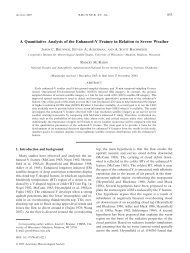
Superobbing vs. Thinning Atmospheric Motion Vectors ... - GOES-R

Patricia Pauley, Nancy Baker, and Rolf Langland
Naval Research Laboratory
Monterey, California
Ninth Annual Symposium on Future Operational Environmental Satellite Systems

FNMOC and GMAO Observation Impact Monitoring
Current Operations
http://www.nrlmry.navy.mil/metoc/ar_monitor/
http://gmao.gsfc.nasa.gov/products/forecasts/sy
stems/fp/obs_impact/
Much larger relative impact of AMVs in Navy system
2

Motivation
Why does NRL/FNMOC appear to obtain more benefit from
AMVs than other NWP centers?
• Superobbing vs. thinning
• Assimilating more winds
• Assimilating geostationary winds from NESDIS/EUMETSAT/JMA and from
CIMSS/AFWA—two datasets for each satellite
• Making separate superobs for each processing center, satellite, and channel
• Assimilating hourly winds where available
• Assimilating fewer satellite radiance obs with less impact

Data Overview—CIMSS/UW Winds

AFWA Winds

NESDIS/EUMETSAT/JMA Winds

NESDIS Hourly Winds

Motivation
In experiments using satwinds processed by NRL in the GMAO
system, Gelaro et al. found:
• NRL AMVs provided a substantially increased beneficial impact
and an improvement in overall forecast skill in the GMAO system,
compared to using the NCEP AMVs.
• The greater volume of NRL AMVs appeared to be the primary
reason for the larger impact.
• Superobbing also appears to be beneficial, although secondary to
the influence of data volume.
• The smaller impact of NRL AMVs in the GMAO system compared
to their impact in the NRL system appears to result from the
larger number of satellite radiances used in the GMAO system.
From “Impact of Satellite Atmospheric Motion Vectors in the GMAO GEOS-5 Global Data Assimilation System”, by Gelaro, Merkova, McCarty, and
Tai, presented at the 5th WMO Workshop on the Impact of Various Observing Systems on NWP, Sedona, AZ, May 2012 .

Objective
Examine the degree to which superobbing provides a benefit
over thinning
• NAVGEM (Navy Global Environmental Model)
• 4DVAR data assimilation system (NAVDAR-AR)
• T359L50 (approx. 35 km resolution), model top at .04 hPa
• Superobbing experiment (FNMOC ops configuration):
• Equal-area prisms (2° lat x 2° lon at the equator), 50 mb deep, within 1 hr
• Obs from the same satellite, channel, processing center used in superobs
• Prisms with winds that vary more than thresholds subjected to outlier
rejection and/or horizontal quartering
• No superobs made in prisms with large variability in the winds
• Thinning experiment:
• Same prisms, ob grouping
• Ob with the highest QI selected from same subset of obs that are used to
form superobs, but without quartering

AMV Superob Processing
• Perform QC on individual observations
• Exclude invalid observations with missing position, time, background
• Exclude observations flagged as bad or having low confidence or quality
• EUMETSAT/JMA confidence value less than provided threshold
• NESDIS QI values less than 60
• CIMSS RFF values less than 40 or CIMSS QI values less than 50
• Impose vertical limits as a function of channel
• Impose land-masking in selected regions
• Exclude exact duplicates
• Exclude winds with large vector innovations (ob minus background)

Land Masking
Winds at land points within the North America, Western Europe, and Australia
latitude-longitude boxes are excluded from use.

AMV Limits on Vector Innovations
Winds having large
vector innovation (ob
minus background
values) magnitudes are
rejected.

AMV Superob Processing
• Bin winds into latitude-longitude “prisms” in 50 mb layers
• Examine obs in a prism layer from a particular satellite, channel,
and processing center, and superob if criteria met
• Speeds (or innovations) within 7-14 m/s depending on speed
• Directions (or innovations) within 20° or u and v within 5 m/s
• At least two AMVs are required in a prism
• Reject 1 or 2 outliers to meet criteria if necessary
• Quarter superob horizontally and attempt superobs in each
quarter if the above is unsuccessful
• Adjust u and v superobs so that the magnitude of the superob
wind vector is equal to the mean speed ob the individual obs

Northern Hemisphere Prism Distribution
Superobs are formed in
“prisms” that are 2° latitude
by 2° longitude at the
equator. Although the
latitudinal extent of each
prism is kept fixed at 2°, the
longitudinal extent is
allowed to vary, keeping the
area of the prisms
approximately equal while
also keeping an integer
number of prisms in a
latitude band.
The circles in this figure at
located at prism centers.

Thinning vs. Superobbing
The goal of this first test is to compare simple thinning to
superobbing without changing the spatial and temporal
distribution of observations and without changing the number
of observations.
• Superobbing experiment—operational processing as
previously described
• Thinning experiment
• Process AMVs to generate superobs as previously described
• Replace each superob by the unrejected observation closest in space to
the superob, selected from the observations that were used to form
the superob

Experiment Results
Results are comparable in terms of 500 mb anomaly correlation, with superobbing (green)
having a slight advantage at longer forecast ranges in the Southern Hemisphere.

The 200mb speed
error is slightly less
negative for
superobbing (green)
compared to
thinning (blue)
except in the tropics
where thinning is
slightly better.

The 850mb speed
error is slightly less
negative for
superobbing (green)
compared to thinning
(blue) in the Northern
Hemisphere, but
thinning is slightly
better in the tropics
and Southern
Hemisphere.

Thinning vs. Superobbing
The goal of this test is to compare ECMWF-style thinning to
superobbing without forcing the spatial and temporal
distribution of observations and the number of observations to
remain the same.
• Superobbing experiment—operational processing as previously
described
• Thinning experiment
• Process AMVs to QC and bin obs into prisms as previously described
• In place of superobbing, select a single ob from each prism containing
obs by choosing the ob with the highest QI value. If more than one ob
has this QI, select the first one.

No appreciable difference in the ob counts or statistics between the two file formats

Spatial Distribution of Superobs
70 .. .. ..
.X 2 . 547
.. .2 2 5QQ6
22 .222 2.
.2. .254.2 .2
.. .44.3QQQ73
. 23 . .. 25 .2QQ538
.. .. . 4.2.3.3.25 3
X 2. ..3. 2. .653554852892 4. 34
..22Q2..2. . 2 .2 . .2..44585X3. 2 42
60 2 . ...342.3.. . .3.2. 2..Q2. 23233..576742 2 24
22 33 .24.2 .3.2.2 4. .28X4X663 . 5
.. . . .34. 2.2.2....3.......2.. ..224555. 3.45
... .3.3 .2 . X 24522... 3.Q22.. 3 2. 243. .224453
22. .X.4. 23. ..2..2.. 2 .2244. ..523465636346783
. 2.. . .. .2222 . 2. 22. 22. .322 . . .4752235332435.5.
2..2 .3. . .. ...43 574. . 3.QQ452. ..2 2 3248755246765.4432
3 . 2 . 22 235Q. 3X44. 2 2344232. .2.432.22546. 5423222
. . . .. 3. 32322.2 4552 ..22 .2322233.. .33 2.22263 2
22 2. ..2. 2.3. 9654222.22. . .2. . 2 .. 22 . X .353.. .
50 . ..... . .... .3 4222Q33. ... . . ..245365 ..
5499. .2 2.2.732. 32. 222.. 2 2 33.73 .43.
.3.32 .. .. . 2.. ...6 .. .22Q3Q 3.. .
.26 .2 2.3 2 22.3.... .. . 22 2Q.233 2 24 . ..22
. . 2.2. . .. .2.2 .. . .22 ..22 . 2.2.2Q343.2 .. .
53 . . . 2 .2. ..223.2 2.. 23. 265433
46 .22 .....223.. . . . 2..Q. 2 2. . ... . .2 44544
262 . 22 23.Q . . .... . X . . .32
.5 .2 .. .22. . 32.. 2 Q.. .. . . . .2.2
2 2... . ...2.. . .2 ...22 X . . . . ..2323.
40 2 2.2 . .2 . 2 2.. 2 .. .. .2. 333 .523
22 . 2 .2 ..2 2. ..2.3... . ..22. 2 . 222.2 . 43.
.. 2322 . . .. . X222... . .222..2.223..24.23. .. .
5.. . . . 2 22. .2. ...2 . .. 55 265.2 27.
. . . ..... . ..222. .5443.5.
. .. ... 3. . 4..42 ..7422345 .2
2 . . 22.2. .. .323 . 233242 33. 34245
. . . .. . 23 .. 3352.4 .. . 35
. . 4 . .43.43. 232 ..2. .2 .
. . 2..2 2..32 .. .35 35222
30 . .2. . ....X2..X2 . 2 ...2.4.2..234.3.. ..653
. . . 3.3 ...3222..2 2 2 2 3222323226452 . 23
. .2 . ..23.2.42 .3232 .. 223343222444. ..
. .2.. 2 . 2422232 . .2 2 342.23..
.233 . 2 23232. . 32
32. ... . 2. . . . 23
2. 2
. 2
342
.22
20 .
Legend:
Q Prism was quartered
X No superob was made
. Isolated ob allowed
In the thinning experiment,
no quartering is performed,
but an ob is selected in
every prism, changing the
details of the spatial
distribution relative to the
superob experiment.

No appreciable difference in the superob counts or statistics between the two file formats

Only small differences in the superob counts and statistics between superobbing and thinni