Description of the 16-QAM simulation.
Description of the 16-QAM simulation.
Description of the 16-QAM simulation.

Create successful ePaper yourself
Turn your PDF publications into a flip-book with our unique Google optimized e-Paper software.
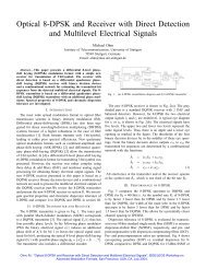
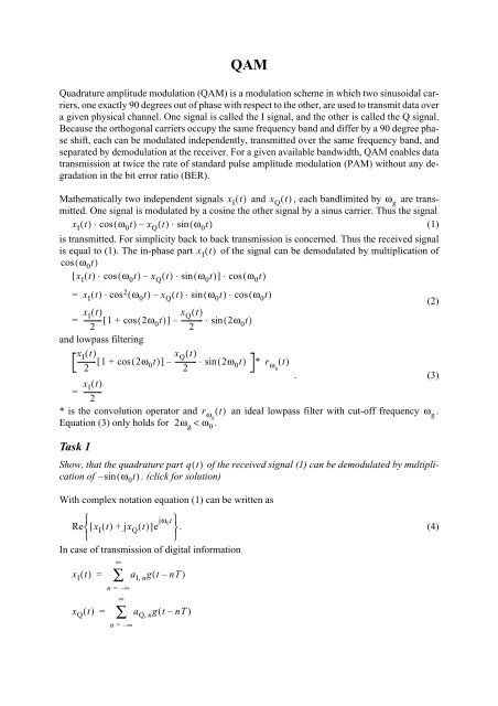
<strong>QAM</strong><br />
Quadrature amplitude modulation (<strong>QAM</strong>) is a modulation scheme in which two sinusoidal carriers,<br />
one exactly 90 degrees out <strong>of</strong> phase with respect to <strong>the</strong> o<strong>the</strong>r, are used to transmit data over<br />
a given physical channel. One signal is called <strong>the</strong> I signal, and <strong>the</strong> o<strong>the</strong>r is called <strong>the</strong> Q signal.<br />
Because <strong>the</strong> orthogonal carriers occupy <strong>the</strong> same frequency band and differ by a 90 degree phase<br />
shift, each can be modulated independently, transmitted over <strong>the</strong> same frequency band, and<br />
separated by demodulation at <strong>the</strong> receiver. For a given available bandwidth, <strong>QAM</strong> enables data<br />
transmission at twice <strong>the</strong> rate <strong>of</strong> standard pulse amplitude modulation (PAM) without any degradation<br />
in <strong>the</strong> bit error ratio (BER).<br />
Ma<strong>the</strong>matically two independent signals x I () t and x Q () t , each bandlimited by ω g are transmitted.<br />
One signal is modulated by a cosine <strong>the</strong> o<strong>the</strong>r signal by a sinus carrier. Thus <strong>the</strong> signal<br />
x I () t ⋅ cos( ω 0 t)<br />
– x Q () t ⋅ sin( ω 0 t)<br />
(1)<br />
is transmitted. For simplicity back to back transmission is concerned. Thus <strong>the</strong> received signal<br />
is equal to (1). The in-phase part x I<br />
() t <strong>of</strong> <strong>the</strong> signal can be demodulated by multiplication <strong>of</strong><br />
cos( ω 0<br />
t)<br />
[ x I<br />
() t ⋅ cos( ω 0<br />
t)<br />
– x Q<br />
() t ⋅ sin( ω 0<br />
t)<br />
] ⋅ cos( ω 0<br />
t)<br />
= x I () t ⋅ cos 2 ( ω 0 t)<br />
– x Q () t ⋅ sin( ω 0 t)<br />
⋅ cos( ω 0 t)<br />
(2)<br />
=<br />
x I<br />
() t<br />
x<br />
---------- Q<br />
() t<br />
[ 1 + cos( 2ω<br />
2<br />
0<br />
t)<br />
] – ------------ ⋅ sin( 2ω<br />
2<br />
0<br />
t)<br />
and lowpass filtering<br />
x I () t<br />
x<br />
---------- Q () t<br />
[ 1+<br />
cos( 2ω<br />
2<br />
0<br />
t)<br />
]– ------------ ⋅ sin( 2ω<br />
2<br />
0<br />
t)<br />
* r ωg<br />
() t<br />
x I () t<br />
= ----------<br />
2<br />
. (3)<br />
* is <strong>the</strong> convolution operator and r ωg<br />
() t an ideal lowpass filter with cut-<strong>of</strong>f frequency ω g .<br />
Equation (3) only holds for 2ω g<br />
< ω 0 .<br />
Task 1<br />
Show, that <strong>the</strong> quadrature part qt () <strong>of</strong> <strong>the</strong> received signal (1) can be demodulated by multiplication<br />
<strong>of</strong> –sin( ω 0<br />
t)<br />
. (click for solution)<br />
With complex notation equation (1) can be written as<br />
⎧<br />
Re [ x I () t + jx Q () t ]e jω 0t ⎫<br />
⎨<br />
⎬. (4)<br />
⎩<br />
⎭<br />
In case <strong>of</strong> transmission <strong>of</strong> digital information<br />
∞<br />
∑<br />
x I () t = a I, n gt ( – nT)<br />
n = – ∞<br />
∞<br />
∑<br />
x Q () t = a Q, n gt ( – nT)<br />
n = – ∞
a n<br />
= a I, n + ja Q,<br />
n . (5)<br />
a n<br />
is <strong>the</strong> complex symbol sequence at <strong>the</strong> output <strong>of</strong> <strong>the</strong> mapper. Thus equation (4) can be written<br />
as<br />
∞<br />
⎧<br />
Re a n<br />
gt ( – nT)e jω 0t ⎫<br />
⎨ ∑<br />
⎬. (6)<br />
⎩<br />
⎭<br />
n = – ∞<br />
Task 2<br />
Show, that with complex notation <strong>the</strong> in-pase and quadrature component <strong>of</strong> <strong>the</strong> modulated signal<br />
(6) can be demodulated by multiplication <strong>of</strong> e jω 0t –<br />
and low-pass filtering. (click for solution)<br />
In <strong>the</strong> following<br />
t = nT, thus<br />
∞<br />
gt ()<br />
is assumed to be a Nyquist impulse with equidistant zero crossings at<br />
⎧<br />
g( 0) Re a n<br />
e jω 0nT ⎫<br />
⋅ ⎨ ∑ ⎬<br />
(7)<br />
⎩n<br />
= – ∞ ⎭<br />
is <strong>the</strong> received signal (6) after sampling. Now additive white gaussian noise (AWGN) is added.<br />
This is depicted in Fig. 1. As sampling and demodulation with ideal low-pass filtering are linear<br />
processes, this will lead to <strong>the</strong> received sequence<br />
g( 0)<br />
ã n<br />
= ----------a (8)<br />
2 n<br />
+ r n<br />
with discrete additive gaussian noise r n<br />
= r I, n + jr Q,<br />
n .<br />
In <strong>the</strong> following <strong>the</strong> impulse gt () is chosen suchlike, that <strong>the</strong> average signal energy<br />
M<br />
1<br />
S = ---- A<br />
2<br />
(9)<br />
M ∑ k<br />
k = 1<br />
and <strong>the</strong> average noise energy<br />
N = E { r 2 } I,<br />
n<br />
= E { r 2<br />
. (10)<br />
Q ,<br />
} = σ 2 n<br />
The decision device has to estimate â n<br />
out <strong>of</strong> ã n<br />
. â n<br />
should be <strong>the</strong> same sequence as a n<br />
. The<br />
influence <strong>of</strong> noise r n<br />
should be as low as possible. r I, n and r Q, n are assumed to be statistically<br />
independent. Thus <strong>the</strong> decision problem can be separated. In case <strong>of</strong> AWGN <strong>the</strong> noise r I,<br />
n and<br />
r Q, n follows <strong>the</strong> probability density function (pdf)<br />
1<br />
1 –-- -----<br />
r2<br />
p I ( r) = p Q ( r)<br />
= -------------- e<br />
2σ 2<br />
, (11)<br />
2πσ<br />
respectively. Thus <strong>the</strong> noise process is normally distributed with zero-mean and variance σ 2 .<br />
In total because real and imaginary part are statistically independent in complex notation<br />
e jω 0t<br />
nt ()<br />
e – jω<br />
0t<br />
low-pass<br />
decision<br />
demapper<br />
b m<br />
mapper a sampler<br />
n<br />
filter device<br />
ã â<br />
+<br />
n bˆ<br />
gt ()<br />
m<br />
× Re{}<br />
×<br />
n<br />
⎧ ⎪⎪⎪<br />
⎪<br />
⎪⎪⎨⎪⎪⎪⎪⎪⎪⎩<br />
⎧ ⎨⎩<br />
⎧ ⎪⎪⎪⎪⎪⎪⎨⎪⎪⎪⎪⎪⎪⎩<br />
transmitter tx AWGN receiver rx<br />
Fig. 1: principle communication system
1 -- ------<br />
pr ( ) = p I<br />
( r I<br />
) ⋅ p Q<br />
( r Q<br />
) = ------------e<br />
2 σ 2<br />
(12)<br />
2πσ 2<br />
is <strong>the</strong> pdf <strong>of</strong> r n<br />
.<br />
For example a four quadrature pulse shift keying (4-QPSK) system is analyzed. Thus<br />
a n<br />
∈ { A 1<br />
= 1 + j, A 2<br />
= 1–<br />
j, A 3<br />
= – 1 + j,<br />
A 4<br />
= – 1 – j}<br />
. Fig. 2 shows this signal constellation.<br />
Task 3<br />
1<br />
– r 2<br />
Calculate <strong>the</strong> average signal energy S 4-QPSK<br />
<strong>of</strong> <strong>the</strong> 4-QPSK. (click for solution)<br />
To this symbols a n<br />
AWGN is added. All four signal points are assumed to occure with <strong>the</strong> same<br />
probability. For simplicity g( 0)<br />
is assumed to be 2.<br />
Task 4<br />
Calculate <strong>the</strong> pdf p ãn<br />
( r) for ã n<br />
. (click for solution)<br />
Fig. 3 shows p ãn<br />
( r)<br />
in a 3-dimensional sketch. This is similar to <strong>the</strong> frequency <strong>of</strong> occurence in<br />
<strong>the</strong> <strong>16</strong>-<strong>QAM</strong> animation, where <strong>the</strong> 3rd dimension is equivalent to <strong>the</strong> density <strong>of</strong> received signal<br />
points, which are plotted in green and red colour. Green stands for correct decision and red for<br />
symbol error.<br />
The decision device has to choose <strong>the</strong> most probable signal point, wich may be sent. If <strong>the</strong> a-<br />
priori probability for <strong>the</strong> signal points is equal as mentioned, <strong>the</strong> decision thresholds consist <strong>of</strong><br />
perpendicular bisectors <strong>of</strong> <strong>the</strong> sides <strong>of</strong> adjacent signal points. That means <strong>the</strong> signal point, which<br />
is most close to <strong>the</strong> received point will be decided to. In this example <strong>the</strong> axes in Fig. 2 are also<br />
<strong>the</strong> decision thresholds.<br />
The probability <strong>of</strong> symbol errors (SER) can be calculated by integration <strong>of</strong> p Ak<br />
( r)<br />
(eq. (23); eg.<br />
Fig. 4) over <strong>the</strong> region in <strong>the</strong> complex r -plane where received symbols ã n<br />
would not be decided<br />
to <strong>the</strong> appropriate sent symbol a n<br />
= A k<br />
, respectively. This has to be done for all k signal<br />
points. The SER is <strong>the</strong> arithmetic average over all.<br />
Im[ A k<br />
]<br />
A 3<br />
1<br />
A 1<br />
1 Re[ A k<br />
]<br />
A 4<br />
A 2<br />
Fig. 2: 4-QPSK constellation
0<br />
∞<br />
1⎛<br />
P 4-QPSK<br />
= -- ⎜ p<br />
4 ∫ ∫ A1<br />
( r)<br />
dr Q<br />
dr I<br />
+ ∫ ∫ p A1<br />
( r)<br />
dr Q<br />
dr I<br />
+ ∫ ∫ p A2<br />
( r)<br />
dr Q<br />
dr I<br />
⎝<br />
–∞ –∞<br />
∞ ∞<br />
∞<br />
0<br />
0 –∞<br />
0<br />
∞<br />
–∞ –∞<br />
+ ∫ ∫ p ( A2<br />
r ) dr Q<br />
dr I<br />
+ ∫ ∫ p A3<br />
( r)<br />
dr Q<br />
dr I<br />
+ ∫ ∫ p A3<br />
( r)<br />
dr Q<br />
dr I<br />
0 0<br />
∞ ∞<br />
∞ ∞<br />
0 –∞<br />
∫ ∫ p ( A4<br />
r ) dr Q dr I ∫ ∫ p A4<br />
r<br />
+ +<br />
0 –∞<br />
0<br />
∞<br />
–∞ 0<br />
⎞<br />
( ) dr Q dr I ⎟<br />
⎠<br />
0<br />
0<br />
–∞ –∞<br />
(13)<br />
0.<strong>16</strong><br />
0.14<br />
0.12<br />
0.1<br />
0.08<br />
0.06<br />
0.04<br />
0.02<br />
0<br />
p ãn<br />
( r)<br />
p ãn<br />
( r)<br />
0.15<br />
0.1<br />
0.0432<br />
0.02<br />
0.01<br />
-2<br />
-1<br />
0<br />
Re[ r]<br />
1<br />
2<br />
-2<br />
-1<br />
0<br />
1<br />
Im[ r]<br />
2<br />
Fig. 3: probability density function <strong>of</strong> ã n<br />
for σ = 0.5<br />
P A1<br />
( r)<br />
0.7<br />
0.6<br />
0.5<br />
0.4<br />
0.3<br />
0.2<br />
0.1<br />
0<br />
P A1<br />
( r)<br />
-2<br />
-1<br />
0<br />
Re[ r]<br />
1<br />
2<br />
-2<br />
-1<br />
0<br />
1<br />
Im[ r]<br />
2<br />
Fig. 4: probability density function <strong>of</strong> ã n<br />
if a n<br />
= A 1<br />
for σ = 0.5
P 4-QPSK<br />
= = ∫ ∫ p A1<br />
( r)<br />
dr Q<br />
dr I<br />
+ ∫ ∫ p A1<br />
( r)dr Q<br />
dr I<br />
= 1–<br />
∫ ∫ p A1<br />
( r)<br />
dr Q<br />
dr I<br />
The simplification in (14) can be done because <strong>of</strong> symmetry. To calculate this integral, <strong>the</strong> separation<br />
<strong>of</strong> (12) can be used.<br />
P 4-QPSK<br />
= 1 –<br />
(14)<br />
In equation (15) <strong>the</strong> substitutions<br />
r<br />
t I/Q<br />
– 1<br />
1 x<br />
= –---------------- and Qx ( ) = -- 1 – erf⎛------<br />
⎞ ⇔ erf( x)<br />
= 1 – 2Q( 2x)<br />
(<strong>16</strong>)<br />
2σ<br />
2 ⎝ 2⎠<br />
are used. With some routine <strong>the</strong> notation with <strong>the</strong> Q-function is very efficient. The Gaussian error<br />
function is defined as<br />
erf( x)<br />
Task 5<br />
Calculate P 4-QPSK as a function <strong>of</strong> SNR (average symbol energy per average noise energy) and<br />
as a function <strong>of</strong> SNRdB (SNR in decibel).<br />
Hint: Scale <strong>the</strong> signal points by a ( A k<br />
= 2a ). adapt <strong>the</strong> result in (15). Normalize adequately.<br />
(click for solution)<br />
Task 6<br />
In Fig. 5 <strong>the</strong> constellation diagram <strong>of</strong> a <strong>16</strong>-<strong>QAM</strong> is depicted. All signal points occure with <strong>the</strong><br />
same probability. Calculate P <strong>16</strong>-<strong>QAM</strong> as a function <strong>of</strong> SNR dB .<br />
Calculate <strong>the</strong> numerical values <strong>of</strong> P <strong>16</strong>-<strong>QAM</strong> for SNR dB = 01234567891011<br />
, , , , , , , , , , , .<br />
Compare your results with <strong>the</strong> calculated values in <strong>the</strong> <strong>16</strong>-<strong>QAM</strong> animation.<br />
Hint: There are three types <strong>of</strong> signal points with different error rate. (click for solution)<br />
Task 7<br />
Give <strong>the</strong> limit <strong>of</strong> SER <strong>of</strong> <strong>the</strong> <strong>16</strong>-<strong>QAM</strong> for very low SNR . (click for solution)<br />
Task 8<br />
0<br />
= 1 –<br />
∞<br />
–∞ –∞<br />
∞ ∞<br />
∫ ∫<br />
0 0<br />
∞<br />
∫<br />
0<br />
1<br />
------------e<br />
2πσ 2<br />
1<br />
-------------- e<br />
2πσ<br />
–∞<br />
– 2<br />
1<br />
–--<br />
r A 1<br />
-------------------<br />
2<br />
σ 2<br />
1( -- r I – A I1 , ) 2<br />
– -------------------------<br />
2<br />
σ 2<br />
∞<br />
0<br />
0 –∞<br />
dr Q<br />
dr I<br />
dr I<br />
⋅<br />
∞<br />
∫<br />
0<br />
1<br />
-------------- e<br />
2πσ<br />
1( -- r Q – A Q1 , ) 2<br />
– -----------------------------<br />
2<br />
Fig. 6 shows a screenshot <strong>of</strong> <strong>the</strong> <strong>16</strong>-<strong>QAM</strong> animation. Only one symbol error occured (red<br />
point). Which signal point was most probably sent? (click for solution)<br />
σ 2<br />
∞ ∞<br />
0 0<br />
dr Q<br />
1<br />
1 –------<br />
e – 1 1<br />
= – ∫<br />
t2 dt 1 --erf ----------<br />
π<br />
2 ⎝<br />
⎛ 2σ⎠<br />
⎞ 1 2<br />
= – + -- = 2Q⎛ 1<br />
2 ⎝σ -- ⎞ – Q<br />
⎠<br />
2 ⎛ 1 ⎝σ -- ⎞<br />
⎠<br />
x<br />
0<br />
1<br />
----------<br />
2σ<br />
2<br />
2<br />
= ------<br />
∫e – x2 dx . (17)<br />
π<br />
(15)
Task 9<br />
Start <strong>the</strong> <strong>16</strong>-<strong>QAM</strong> animation with SNR dB ≈ 20dB . Wait until more than 10 errors (red points)<br />
occured. Make sure, <strong>the</strong>y agglomerate at <strong>the</strong> decision thresholds.<br />
Gray coding is a coding scheme where adjacent signal points differ only by one bit in coding.<br />
Why is this coding scheme useful for <strong>QAM</strong> modulation?<br />
What about low SNR ? (click for solution)<br />
Im[ A k<br />
]<br />
3a<br />
A 1<br />
A 2<br />
A 3<br />
A 4<br />
a<br />
A 5<br />
A 6<br />
A 7 A 8<br />
a<br />
3a<br />
Re[ A k<br />
]<br />
A 9<br />
A 10<br />
A 11<br />
A 12<br />
A 13<br />
A 14<br />
A 15<br />
A <strong>16</strong><br />
Fig. 5: <strong>16</strong>-<strong>QAM</strong> constellation<br />
Fig. 6: Screenshot <strong>of</strong> <strong>the</strong> <strong>16</strong>-<strong>QAM</strong> animation
Solution 1 (click to go back)<br />
–[ x I () t ⋅ cos( ω 0 t)<br />
– x Q () t ⋅ sin( ω 0 t)<br />
] ⋅ sin( ω 0 t)<br />
= – x I () t ⋅ sin( ω 0 t)<br />
⋅ cos( ω 0 t)<br />
+ x Q () t ⋅ sin 2 ( ω 0 t)<br />
x I<br />
() t<br />
x<br />
---------- Q<br />
() t<br />
= – ⋅ sin( 2ω<br />
2<br />
0<br />
t)<br />
+ ------------ [ 1 – cos( 2ω<br />
2<br />
0<br />
t)<br />
]<br />
After lowpass filtering (* is <strong>the</strong> convolution operator):<br />
x I<br />
() t<br />
x<br />
---------- Q<br />
() t<br />
– ⋅ sin( 2ω<br />
2<br />
0<br />
t)<br />
+ ------------ [ 1 – cos( 2ω<br />
2<br />
0<br />
t)<br />
] * r ωg<br />
() t<br />
x Q<br />
() t<br />
= ------------<br />
2<br />
(click to go back)<br />
(18)<br />
(19)
Solution 2 (click to go back)<br />
1<br />
With Re{ z}<br />
= -- ( z + z)<br />
, whereby z is <strong>the</strong> conjugate complex number <strong>of</strong> z , after mutliplication<br />
– 2<br />
<strong>of</strong> e jω 0t<br />
∞<br />
⎧<br />
Re a n<br />
gt ( – nT)e jω 0t ⎫ – jω 0 t<br />
⎨ ∑<br />
⎬⋅<br />
e<br />
⎩<br />
⎭<br />
n = – ∞<br />
∞<br />
1<br />
-- a<br />
2 n e jω 0t –<br />
a n e jω 0t<br />
–<br />
( + )gt ( – nT) e jω 0t<br />
= ∑<br />
⋅<br />
n = – ∞<br />
∞<br />
1<br />
–<br />
-- a<br />
2 n<br />
a n<br />
e j2ω 0t<br />
= ∑ ( + )gt ( – nT)<br />
n = – ∞<br />
and after lowpass filtering (20) gets<br />
∞<br />
1<br />
–<br />
-- a<br />
2 n<br />
a n<br />
e j2ω 0t<br />
∑ ( + )gt ( – nT )<br />
1<br />
* r ωg<br />
() t = -- a<br />
2 ∑ n<br />
gt ( – nT)<br />
n = – ∞<br />
(click to go back)<br />
∞<br />
n = – ∞<br />
(20)<br />
(21)
Solution 3 (click to go back)<br />
4<br />
1<br />
S 4-QPSK<br />
-- A 2 1<br />
=<br />
4 ∑ k<br />
= -- ( 1 + j<br />
4<br />
+ 1 – j<br />
+ – 1 + j<br />
+ – 1 – j<br />
) =<br />
k = 1<br />
2 . (22)<br />
The signal and noise power do not have units, because <strong>of</strong> standardization!<br />
(click to go back)
Solution 4 (click to go back)<br />
p ãn<br />
4<br />
1<br />
( r)<br />
= -- p<br />
4 ∑ Ak<br />
( r)<br />
=<br />
k = 1<br />
(click to go back)<br />
1<br />
--<br />
4<br />
4<br />
∑<br />
k = 1<br />
1<br />
------------e<br />
2πσ 2<br />
– 2<br />
1<br />
–--<br />
r A k<br />
------------------<br />
2<br />
σ 2<br />
(23)
Solution 5 (click to go back)<br />
With <strong>the</strong> new signal points A 1<br />
= a + ja ; A 2<br />
= a – ja ; A 3<br />
= – a + ja ; A 4<br />
= – a – ja <strong>the</strong><br />
average signal energy<br />
S 4-QPSK = 2a 2 . (24)<br />
Thus <strong>the</strong> SER gets<br />
P 4-QPSK<br />
2Q⎛ a ⎝σ -- ⎞ Q<br />
⎠<br />
– 2 ⎛ a ⎝σ -- ⎞<br />
⎠<br />
2Q ⎛------<br />
1 2a 2<br />
2<br />
-------- ⎞<br />
⎝ σ 2 Q<br />
⎠<br />
2 1<br />
= =<br />
– ⎛------<br />
⎝ 2<br />
2a<br />
--------<br />
2 ⎞<br />
⎠<br />
SNR dB<br />
SNR .<br />
= 2Q<br />
SNR ----------<br />
⎝<br />
⎛ 2 ⎠<br />
⎞ – Q2 ⎛ SNR ---------- ⎞ 2Q 10 ---------------<br />
dB<br />
⎛<br />
10<br />
⎞ ⎛ ---------------<br />
⎜ ------------------ ⎟ Q<br />
⎝ 2 ⎠ ⎜ 2 ⎟<br />
2 10<br />
10<br />
⎞<br />
=<br />
– ⎜ ------------------ ⎟<br />
⎜ 2 ⎟<br />
⎝ ⎠ ⎝ ⎠<br />
(click to go back)<br />
σ 2
Solution 6 (click to go back)<br />
S <strong>16</strong>-<strong>QAM</strong> = 10a 2<br />
(25)<br />
4<br />
P <strong>16</strong>-<strong>QAM</strong> = ----- 2Q⎛ a<br />
<strong>16</strong> ⎝σ -- ⎞ – Q<br />
⎠<br />
2 ⎛ a ⎝σ -- ⎞<br />
⎠<br />
⎧ ⎪⎪⎪⎨⎪⎪⎪⎩<br />
A 1<br />
, A 4<br />
, A 13<br />
, A <strong>16</strong><br />
+<br />
8<br />
----- Q⎛ a<br />
<strong>16</strong> ⎝σ -- ⎞ ⎧<br />
+ 1 – Q⎛ a<br />
⎠ ⎝σ -- ⎞<br />
⎨ ⎠<br />
⎩<br />
⎧ ⎪⎪⎪⎪⎪⎪⎪⎨⎪⎪⎪⎪⎪⎪⎪⎩<br />
⎫ ⎧<br />
⎬⋅<br />
⎨<br />
⎭ ⎩<br />
⎛ ⎞ Q⎛ a ⎝σ -- ⎞⎫<br />
+<br />
⎠⎬<br />
⎭<br />
Q a σ -- ⎝ ⎠<br />
A 2<br />
, A 3<br />
, A 5<br />
, A 8<br />
, A 9<br />
, A 12<br />
, A 14<br />
, A 15<br />
+<br />
4<br />
----- 2Q⎛ a<br />
<strong>16</strong> ⎝σ -- ⎞ ⎧<br />
+ 1–<br />
2Q⎛ a<br />
⎠ ⎝σ -- ⎞<br />
⎨ ⎠<br />
⎩<br />
⎧ ⎪⎪⎪⎪⎪⎪⎨⎪⎪⎪⎪⎪⎪⎩<br />
A 6<br />
, A 7<br />
, A 10<br />
, A 11<br />
⎫ a<br />
⎬⋅<br />
2Q --<br />
⎝ ⎛ ⎭ σ⎠<br />
⎞<br />
(26)<br />
3Q⎛ a ⎝σ -- ⎞ 9<br />
= – --Q<br />
⎠ 4<br />
2 ⎛ a ⎝σ -- ⎞ 3Q⎛ SNR ---------- ⎞ 9<br />
=<br />
– --Q<br />
⎠ ⎝ 10 ⎠ 4<br />
2 ⎛<br />
⎝<br />
SNR<br />
---------- ⎞<br />
10 ⎠<br />
=<br />
⎛<br />
3Q⎜<br />
⎜<br />
⎝<br />
SNR dB<br />
10 ---------------<br />
10<br />
⎞<br />
------------------ ⎟<br />
10 ⎟<br />
⎠<br />
–<br />
SNR dB<br />
⎛ ---------------<br />
9<br />
--Q<br />
4<br />
2 10<br />
10<br />
⎞<br />
⎜ ------------------ ⎟<br />
⎜ 10 ⎟<br />
⎝ ⎠<br />
(27)<br />
SNR dB<br />
P <strong>16</strong>-<strong>QAM</strong><br />
SNR dB<br />
P <strong>16</strong>-<strong>QAM</strong><br />
0 0.80979256 12 0.28773651<br />
1 0.79027909 13 0.22268236<br />
2 0.76759250 14 0.<strong>16</strong>230454<br />
3 0.74125244 15 0.10984263<br />
4 0.71074913 <strong>16</strong> 0.067830428<br />
5 0.67557021 17 0.037404624<br />
6 0.63524598 18 0.017932041<br />
7 0.58941918 19 0.0072268271<br />
8 0.53794439 20 0.0023467250<br />
9 0.48101796 21 0.00058187175<br />
10 0.41932991 22 0.00010290522<br />
11 0.35421249 23 0.000011907710<br />
(click to go back)
Solution 7 (click to go back)<br />
15<br />
In case <strong>of</strong> very low SNR all signal points are equal probable. Thus P <strong>16</strong>-<strong>QAM</strong> → -----<br />
<strong>16</strong><br />
(click to go back)<br />
= 0.9375
Solution 8 (click to go back)<br />
Signal point A 13<br />
was most probably sent, because it is <strong>the</strong> second most close signal point to <strong>the</strong><br />
received signal point (red point).<br />
(click to go back)
Solution 9 (click to go back)<br />
In case <strong>of</strong> gray coding most symbol errors lead to only one bit error, because most wrong decided<br />
symbols come from adjacent signal points and <strong>the</strong> coding <strong>of</strong> <strong>the</strong>m differ only by one bit.<br />
Thus approximately if M bits are transmitted per symbol <strong>the</strong> bit error ratio (BER) is equal to<br />
P SER<br />
P BER<br />
≈ ----------- . (28)<br />
M<br />
This only holds for high SNR . In case <strong>of</strong> low SNR a lot <strong>of</strong> wrong decided symbols come from<br />
signal points far away. The advatage <strong>of</strong> gray coding vanishs.<br />
(click to go back)