Discolouration in drinking water systems - TU Delft
Discolouration in drinking water systems - TU Delft
Discolouration in drinking water systems - TU Delft

You also want an ePaper? Increase the reach of your titles
YUMPU automatically turns print PDFs into web optimized ePapers that Google loves.
flow direction is decreas<strong>in</strong>g. At the end of the measur<strong>in</strong>g period at location 2 there is an<br />
<strong>in</strong>crease <strong>in</strong> turbidity that is not related to the turbidity at the treatment plant and is probably<br />
caused by a resuspension of settled material. That is <strong>in</strong> accordance with the observation that<br />
for the majority of time the turbidity drops <strong>in</strong>dicat<strong>in</strong>g that material is lost from the fluid and<br />
probably settl<strong>in</strong>g at the pipe wall. An <strong>in</strong>crease <strong>in</strong> velocity will <strong>in</strong>crease the sheer stress and<br />
resuspend the settled material.<br />
If these locations were monitored with samples, then it would be impossible to analyse the<br />
process of regular settl<strong>in</strong>g and resuspension of material. Samples are mostly taken dur<strong>in</strong>g<br />
office hours, so the 24-hour <strong>in</strong>formation on the pattern will be lost. Moreover at the network<br />
locations the levels of turbidity also vary on a shorter time scale with short <strong>in</strong>creases. Those<br />
are represented by the short spikes <strong>in</strong> read<strong>in</strong>gs. Given the scale of the time axis, these spikes<br />
last for at least half an hour. The chance that samples are taken dur<strong>in</strong>g those short spikes is<br />
unrealistic and that would leave the phenomena unclear.<br />
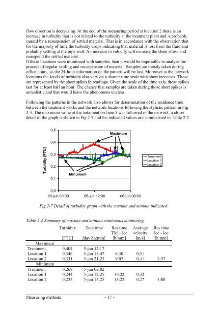
Follow<strong>in</strong>g the patterns <strong>in</strong> the network also allows for determ<strong>in</strong>ation of the residence time<br />
between the treatment works and the network locations follow<strong>in</strong>g the stylistic pattern <strong>in</strong> Fig<br />
2-3. The maximum value at the tretament on June 5 was followed <strong>in</strong> the network; a closer<br />
detail of the graph is shown <strong>in</strong> Fig 2-7 and the <strong>in</strong>dicated values are summarised <strong>in</strong> Table 2-2.<br />
0,5<br />
Maximum<br />
0,4<br />
Turbidity [F<strong>TU</strong>]<br />
0,3<br />
0,2<br />
0,1<br />
M<strong>in</strong>umum<br />
Treatment<br />
Location 1<br />
Location 2<br />
0,0<br />
05-jun 00:00 05-jun 12:00 06-jun 00:00<br />
Fig 2-7 Detail of turbidity graph with the maxima and m<strong>in</strong>ima <strong>in</strong>dicated<br />
Table 2-2 Summary of maxima and m<strong>in</strong>ima cont<strong>in</strong>uous monitor<strong>in</strong>g<br />
Turbidity Date time Res time Average Res time<br />
TM – loc velocity loc - loc<br />
[F<strong>TU</strong>] [day hh:mm] [h:mm] [m/s] [h:mm]<br />
Maximum<br />
Treatment 0,404 5-jun 12:17<br />
Location 1 0,346 5-jun 18:47 6:30 0,51<br />
Location 2 0,331 5-jun 21:25 9:07 0,41 2:37<br />
M<strong>in</strong>imum<br />
Treatment 0,269 5-jun 02:02<br />
Location 1 0,244 5-jun 12:25 10:22 0,32<br />
Location 2 0,235 5-jun 15:25 13:22 0,27 3:00<br />
Measur<strong>in</strong>g methods - 17 -