Exercises - Isabelle MEJEAN's home page

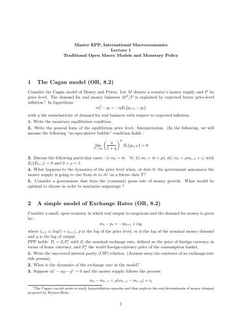
Master EPP, International Macroeconomics
Lecture 1
Traditional Open Macro Models and Monetary Policy
1 The Cagan model (OR, 8.2)
Consider the Cagan model of Money and Prices. Let M denote a country’s money supply and P its
price level. The demand for real money balances M d /P is explained by expected future price-level
inflation. 1 In logarithms:
m d t − p t = −ηE t {p t+1 − p t }
with η the semielasticity of demand for real balances with respect to expected inflation.
1. Write the monetary equilibrium condition.
2. Write the general form of the equilibrium price level. Interpretation. (In the following, we will
assume the following “no-speculative bubble” condition holds :
( ) η T
lim
E t {p t+T } = 0
T →∞ 1 + η
3. Discuss the following particular cases : i) m t = ¯m ∀t, ii) m t = ¯m + µt, iii) m t = ρm t−1 + ε t with
E t {E t+1 } = 0 and 0 < ρ < 1.
4. What happens to the dynamics of the price level when, at date 0, the government announces the
money supply is going to rise from ¯m to ¯m ′ on a future date T ?
5. Consider a government that fixes the (constant) gross rate of money growth. What would be
optimal to choose in order to maximize seignorage ?
2 A simple model of Exchange Rates (OR, 8.2)
Consider a small, open economy in which real output is exogenous and the demand for money is given
by:
m t − p t = −ηi t+1 + φy t
where i t+1 ≡ log(1 + i t+1 ), p is the log of the price level, m is the log of the nominal money demand
and y is the log of output.
PPP holds: P t = E t Pt
∗ with E t the nominal exchange rate, defined as the price of foreign currency in
terms of home currency, and Pt
∗ the world foreign-currency price of the consumption basket.
1. Write the uncovered interest parity (UIP) relation. (Assume away the existence of an exchange-rate
risk premia)
2. What is the dynamics of the exchange rate in the model?
3. Suppose ηi ∗ − φy − p ∗ = 0 and the money supply follows the process:
m t − m t−1 = ρ(m t−1 − m t−2 ) + ε t
1 The Cagan’s model seeks to study hyperinflation episodes and thus neglects the real determinants of money demand
proposed by Keynes-Hicks.
1

where ε is a serially uncorrelated mean-zero shock such that E t−1 {ε t } = 0. Write the dynamics of the
exchange rate.
4. Assume now that the government wishes to fix the (log of the) nominal exchange rate permanently
at ē. What path of the money supply is consistent with having e t = ē permanently?
4. During the beginning of the US Reagan administration in 1981, some US officials seriously discussed
the possibility of making a transition to a fixed exchange rate for the dollar. However, they argued
that it would be presumptuous for government officials to decide the best exchange rate and that they
should instead let the market decide. The policy they proposed was to announce today that at some
future date T they would permanently fix the exchange rate (using monetary policy) at whatever level
prevailed in the market at time T − 1. Is this a coherent policy?
3 The Mundell-Fleming-Dornbusch model (OR, 9.2)
Consider a small open economy facing an exogenous world (foreign-currency) interest rate i ∗ . With
open capital markets and perfect foresight, uncovered interest parity holds. Only domestic residents
holds the domestic money, according to the following relationship:
m t − p t = φy t − ηi t+1 (1)
where m t , p t and y t respectively denote the log of nominal money demand, the price level and output
and i t+1 = log(1 + i t+1 ). The Purchasing Power Parity needs not hold so that the real exchange rate
q t = e t + p ∗ t − p t can vary. (In the following, the foreign price p ∗ is assumed constant.)
The Dornbusch model effectively aggregates all domestic output as a single composite commodity and
assumes that aggregate demand for home-country output, y d , is equal to:
y d t = ȳ + δ(q t − ¯q), δ > 0 (2)
where ȳ is the “natural” rate of output and ¯q the “equilibrium” real exchange rate consistent with
full-employment. For simplicity, ȳ and ¯q are assumed to be constant.
Prices are rigid in the short-run and flexible in the long-run. Namely, p t is assumed to be predetermined
so that unanticipated shocks can lead to excess demand or supply. In the Keynesian
tradition, it is assumed that output is demand determined. The price level adjusts according to the
inflation-expectations-augmented Phillips curve:
p t+1 − p t = ψ(y d t − ȳ) + (˜p t+1 − ˜p t ) (3)
where ˜p t ≡ e t + p ∗ t − ¯q t is the price level that would prevail if the output market cleared.
In the following, it is assumed that ψδ < 1 which assures a monotonic adjustment of the real exchange
rate. To simplify, the following normalizations are also assumed: p ∗ = ȳ = i ∗ = 0.
1. Interpret the assumption δ > 0 in equation (??).
2. Interpret equation (??).
3. Assume that money supply is constant (m t = ¯m). What is the the dynamics of the nominal and
real exchange rates?
4. What is the impact of an unanticipated permanent rise in the money demand at date 0?
5. Consider now the same model with ȳ ≠ 0. Discuss and show graphically (and partially analytically)
the short- and long-run effects of a rise in natural output.
2