Lecture 5 - Isabelle MEJEAN's home page

Betts & Devereux (1996) 

Campa & Goldberg (2006) 

Lecture 5: Pricing to market and exchange rate 

pass through: empirics and theory 

Isabelle Méjean 

isabelle.mejean@polytechnique.edu 

http://mejean.isabelle.googlepages.com/ 

Master Economics and Public Policy, International Macroeconomics 

November 13 th , 2008 

Isabelle Méjean Lecture 5



Pricing-to-Market and Exchange Rate 

Pass-through 



Motivation 



Try to explain the low impact of exchange rate movements on prices 

of traded goods (incomplete ERPT) 

In traditional models: P M t = E t ∗ P X t Any change in E t is fully 

reflected into import prices (expressed in the importer’s currency) → 

Change the relative price of imported goods → Expenditure 

switching effect (justifies flexible exchange rate regimes) 

In the data, import prices are unsensitive to exchange-rate shocks, at 

least in the short term 

Important consequences concerning the impact of exchange rate 

fuctuations and the optimality of flexible exchange rate regimes 

⇒ Understanding the sources of incomplete pass-through has been a 

major concern in international macroeconomics over the last 10 

years. 


Intuition 



Betts & Devereux allow for PTM in a general equilibrium framework 

with sticky prices 

Pricing-to-Market: see Krugman (1987) and Dornbusch (1987). 

Exchange-rate fluctuations affecting the local price of exported 

goods may induce exporters to set different (FOB) prices in different 

export markets in order to smooth the impact of ER fluctuations 

In the paper, PTM is introduced by assuming that some firms set 

their price in their own currency (PCP) while some firms prefer 

fixing their export price directly in the importer’s currency (LCP) 

When ERs fluctuate and prices are sticky, PCP implies full 

pass-through (as Pt 

M = E t ∗ ¯P t X ) while LCP implies no pass-through 

(as ¯P t 

M = E t ∗ Pt X ). Under LCP, the ER risk is transferred on the 

firm’s mark-up while under PCP, it transmits into a risk of demand. 

In general equilibrium, incomplete ERPT implies that exchange rates 

must adjust more strongly following an asymmetric shock → 

Explains the high volatility of RERs with respect to the volatility of 

NERs. 


Hypotheses 



Two country economy 

International markets are segmented → Consumers cannot without 

significant cost directly arbitrage between price differences across 

countries 

Prices are sticky → Don’t adjust instantaneously to money shocks 

Product are differentiated: 

[∫ 1 

C = 

0 

] σ 

c(i) σ−1 σ−1 

σ di 

Households supply labour, consume and value real money: 

( 

U = logC + 

γ ( ) 1−ɛ M 

+ ηlog(1 − h)) 

1 − ɛ P 

A share n of products are produced in the domestic country 

A share s of exporting firms sets their price under LCP 

Linear technology function: y(i) = Ah(i) 




Households’ behaviour 

Households solve the following 2-step program: 

{ ( 

max C,h,M logC + 

γ ( M 

) 1−ɛ 

) 

1−ɛ P + ηlog(1 − h) 

s.t. PC + M = Wh + π + M 0 + TR 

⎧ 

⎨ 

⎩ 

max C(i) 

[ ∫ 1 

0 

) σ 

σ−1 σ−1 

c(i) σ di 

s.t. PC = ∫ 1 

0 v(i)c(i)di 

where v(i) is the price of variety i, either p(i) if i ∈ [0; n] or p ∗ (i) if 

i ∈ [n; n + (1 − n)s] or eq(i) ∗ if i ∈ [n + (1 − n)s; 1]. 




Households’ behaviour (2) 

Optimality conditions: 

Ideal price index: 

P = 

[ ∫ n 

0 

( 

1 M 

C = γ P 

η 

1 − h = W PC 

( v(i) 

c(i) = 

P 

) −ɛ 

) −σ 

∫ n+(1−n)s 

∫ ] 1 

1 

1−σ 

p(i) 1−σ di + p ∗ (i) 1−σ + (eq ∗ (i)) 1−σ di 

n 

n+(1−n)s 

The situation of foreign households is entirely analogous. 




Firms’ behaviour 

LCP firms solve the following program: 

⎧ 

⎪⎨ 

⎪⎩ 

max p(i),q(i) π LCP (i) = p(i)c(i) + eq(i)c ∗ (i) − W A (c(i) + c∗ (i) 

( ) −σ 

s.t. c(i) = p(i) 

P nC 

( ) −σ 

c ∗ (i) = q(i) 

P (1 − n)C 

∗ 

∗ 

Optimal prices are thus given by: 

p(i) = 

q(i) = 

σ W 

σ − 1 A 

σ W 

σ − 1 Ae 

Under flexible prices, the law of one price holds: p(i) = eq(i). 




Firms’ behaviour (2) 

PCP firms solve the following program: 

⎧ 

⎪⎨ 

⎪⎩ 

max p(i) π PCP (i) = p(i)c(i) + p(i)c ∗ (i) − W A (c(i) + c∗ (i) 

( ) −σ 

s.t. c(i) = p(i) 

P nC 

( ) −σ 

c ∗ (i) = p(i) 

eP (1 − n)C 

∗ 

∗ 

Optimal price is: 

p(i) = 

σ W 

σ − 1 A 

The law of one price holds under flexible prices and under sticky 

prices. 




Aggregate prices 

PPP holds under flexible prices 

P = 

P ∗ = 

" 

σ W 1−σ 

σ W ∗ 1−σ 

n 

+ (1 − n)s e 

(1 − n)(1 − s) e 

σ − 1 A 

σ − 1 A ∗ 

" 

σ W 1−σ 1 σ W 

ns 

+ n(1 − s) 

σ − 1 Ae 

e σ − 1 A 

1−σ 

(1 − n) 

σ 

σ − 1 

σ 

σ − 1 

W ∗ 

A ∗ 1−σ 

W ∗ # 1 

1−σ 1−σ 

A ∗ 

⇒ P = eP ∗ 

PPP does not hold under sticky prices when some firms price in LCP: 

⇒ 

ˆP = (1 − n)(1 − s)ê 

ˆP ∗ = −n(1 − s)ê 

ˆP − ˆP ∗ = (1 − s)ê ≠ ê 




Exchange-rate dynamics 

ê(1 − s) = ( ˆM − ˆM ∗ ) − 1 ɛ (Ĉ − Ĉ ∗ ) 

Exchange rate depreciates in response to relative national money 

growth, and appreciates in response to relative national growth in 

real consumption. 

The size of s determines the magnitude of the departure from PPP 

and of the exchange-rate adjustment to shocks. 


Conclusion 



Under flexible nominal prices, PTM has no aggregate implications 

for any kinds of shocks and PPP holds: eP ∗ = P 

Deviations from PPP are explained by the combination of sticky 

prices and PTM 

PTM as a reversed effect on the way exchange-rates adjust to 

monetary shocks 

⇒ Important consequences on the way open economics adjust to 

asymmetric shocks. 

Limit: Incomplete ERPT explained by sticky prices → Full 

pass-through in the long-run → Empirical evidence rather suggests 

that ERPT is incomplete, even in the long-run → There must be 

some incentive to PTM, beyond the impact of SR ER fluctuations 

→ Models in which firms have an incentive to PTM (Corsetti & 

Dedola, etc.) 




Distribution Margins, Imported Inputs, and 

the Sensitivity of the CPI to Exchange Rates 



Motivation 



Border prices of traded goods are highly sensitive to exchange rates, 

but the CPI, and the retail prices of these goods, are more stable. 

The paper builds a model explaining these differences in exchange 

rate pass-through to import prices and consumer prices. 

⇒ Important roles of local distribution margins and imported inputs in 

transmitting exchange rate fluctuations into consumption prices. 

Empirical analysis based on data for twenty-one OECD countries 

comparing distribution margins, imported inputs and weights in 

consumption of nontradables, home tradables and imported goods 

across countries and industries. 

⇒ Calibration exercise allowing to compute the predicted ERPT into 

CPI for different countries (comparable with existing estimates) 




Overview of results 

⇒ While distribution margins damp the sensitivity of consumption 

prices of tradable goods to exchange rates, they also lead to 

enhanced pass through when nontraded goods prices are sensitive to 

exchange rates. Such price sensitivity arises because imported inputs 

are used in production of home nontradables. 

Calibration exercises show that, at under 5 percent, the United 

States has the lowest expected CPI sensitivity to exchange rates of 

all countries examined. On average, calibrated exchange rate pass 

through into CPIs is expected to be closer to 15 percent. 

⇒ Consistent with empirical estimates of aggregate ERPTs 




ERPT into import and consumer price indices 

Use quarterly data for the period 1975:1 to 2003:4 

Estimated equation: 

∆p it = α∆e it + β∆p ∗ t 

where p is either the log of the import price index or the log of the 

CPI in country i, e is the effective exchange rate and p ∗ is a 

measure of foreign price. Under complete ERPT, α = 1 

Add lags to account for partial price adjustments ⇒ ERPT defined 

as the cumulative one-year impact from an exchange rate shock (LR 

ERPT) 




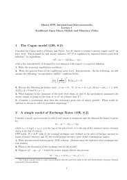
Table 1: Exchange Rate Pass-through Elasticities into Import and Consumer 

Price Indices 

Country 

Pass-Through on Import 

Prices 

Pass-through on Consumer 

Prices 

Australia 0.67*+ 0.09+ 

Austria 0.10 -0.09 

Belgium 0.68 0.08+ 

Canada 0.65*+ -0.01+ 

Czech Republic 0.6* 0.60*+ 

Denmark 0.82* 0.16*+ 

Finland 0.77 -0.02+ 

France 0.98* 0.48*+ 

Germany 0.80* 0.07+ 

Hungary 0.78* 0.42*+ 

Ireland 0.06 0.08+ 

Italy 0.35+ 0.03+ 

Japan 1.13* 0.11*+ 

Netherlands 0.84* 0.38*+ 

New Zealand 0.22+ -0.10*+ 

Norway 0.63* 0.08+ 

Poland 0.78* 0.59*+ 

Portugal 1.08* 0.60*+ 

Spain 0.70* 0.36*+ 

Sweden 0.38*+ -0.11+ 

Switzerland 0.93* 0.17*+ 

United Kingdom 0.46*+ -0.11+ 

United States 0.42*+ 0.01+ 

Average 0.64 0.17 

* (+) indicates exchange rate pass through significantly different from zero (one) at a 5 percent 

confidence level. Most data are quarterly, spanning 1975 through early 2003. Data sources: nominal 

exchange rate and consumer prices come from the IFS; import price comes from the OECD. Specific 

start and end dates by country are detailed in the data appendix. Long-run elasticities (four quarters) 

shown. 




ERPT into import and consumer price indices (3) 

Difference between the import price and the CPI responsiveness to 

exchange rate movements for almost all OECD countries ⇒ Pass 

through into border prices far exceeds pass through into the CPI. 

The (unweighted) average pass through elasticity is 0.64 for import 

prices. It is significantly different from zero in seventeen of the 

twenty-three countries. VERIFIER LA DEFINITION DES PRIX 

The average pass-through into consumer prices is 0.17 over the long 

run. These averages mask huge cross-country differences in CPI 

sensitivity. Nevertheless, the hypothesis that the pass through to 

CPIs is smaller than one can be rejected for all but one country. In 

general, larger countries tend to have lower levels of estimated pass 

through into the CPI. 




Intuition for the low ER sensitivity of CPIs 

CPIs aggregate traded and non-traded goods. Only tradables are 

expected to be sensitive to ERs 

The retail price of traded goods contains non-traded components: 

Expenditures on transportation, storage, finance, insurance, 

wholesaling, and retailing add local-value-added components to the 

final consumption value of imports. 

There can be “double marginalization”: distributors may have an 

incentive to absorb some of the exchange-rate fluctuations in order 

to maintain stable prices or expand market share at the retail level 


Hypotheses 



Two country model with wage stickiness (wages are sticky over the 

relevant pricing horizon) 

Imported inputs in the production of tradable and nontradable goods 

⇒ Producing costs sensitive to exchange rates 

Distribution costs in terms of nontradables ⇒ Failure of purchasing 

power parity due to the presence of local transaction and distribution 

costs. 




Hypotheses (2): Consumption structure 

C.E.S. utility functions over nontraded and traded goods 

consumption: 

C = 

[α 1 Φ C 

Φ−1 

Φ 

T 

+ (1 − α) 1 Φ−1 

] Φ 

Φ−1 

Φ C 

Φ 

N 

Home (h) and foreign (f) tradable goods consumption are imperfect 

substitutes: 

[ 

1 Φ 

Φ 

C T = α T 

T 

C T −1 

Φ T 

TH 

+ (1 − α T ) 1 Φ T −1 

] Φ T 

Φ T −1 

Φ 

Φ 

T C T 

TF 

Both sectors produce a continuum of varieties with similar 

elasticities of substitution: 

[∫ 1 

] θ 

C N = c(n) θ−1 θ−1 

θ dn 

0 

[∫ 1 

C TH = 

0 

] θ 

c(h) θ−1 θ−1 

θ dh 




Hypotheses (3): Supply side 

The marginal cost has two components: the production cost and the 

distribution cost. 

Bringing one unit of traded goods to consumers requires units of a 

basket of differentiated nontraded goods: 

MC t (h) = PC t (h) + m t (h)P Nt 

with PC t (h) the cost of producing variety h at producer level, 

[ ∫ ] 1 

m t (h) = 

0 m θ−1 θ 

θ−1 

θ 

n dn the basket of nontraded inputs and PNt 

the ideal price index for non-traded inputs. 

Per unit production requires imported input share µ t (h) on home 

tradable goods and µ t (n) on home nontradable goods 





Maximizing profits given optimal demands gives: 

θ 

p t (h) = 

[µ t (h) e tW ∗ 

+ W ] 

+ m t (h)P Nt 

θ − 1 Z F Z H 

θ 

p t (n) = 

[µ t (n) e tW ∗ 

+ W ] 

θ − 1 Z F Z N 

[ 

θ et W ∗ 

] 

p t (f ) = 

+ m t (f )P Nt 

θ − 1 Z F 

with Z exogenous sector-specific praoductivity parameters and e t 

domestic currency price of foreign currency. 

No imported inputs in the production of foreign varieties? 

Imported inputs are homogeneous? 

No distribution costs for nontradables? (Useless in explaining ERPT) 





Possibility of double marginalization: 

The distribution margin m t (i), i = h/f is possibly sensitive to 

exchange rates ⇒ Allows for possible deviations from the 

competitive distribution sector assumed in the model 

Exchange rate sensitivity of import shares: 

Imported input shares, µ t (i), i = h/n can be sensitive to exchange 

rate movements ⇒ Incomplete ERPT on imported inputs or 

sensitivity of the local content to exchange rates. 




Pass-through rates at the good level 

η p(n) 

e = 

η p(h) 

e = 

θ 

(1 + ηµ(n) e ) µ t(n) etW ∗ 

Z F 

θ − 1 p t (n) 

[ 

θ 

(1 + η e 

µ(h) ) µ t(h) etW ∗ 

Z F 

θ − 1 

p t (h) 

+ (η m(h) 

e 

ηe p(f ) = 1 − θ m t (f )P 

[ 

] 

Nt 

1 − (ηe 

m(f ) + ηe P(n) ) 

θ − 1 p t (f ) 

+ ηe 

P(n) ) m t(h)P Nt 

p t (h) 

Remark: Implicitely assumes that all η are constant over time. 

] 




Pass-through rates at the good level (2) 

Non-traded goods are sensitive to exchange rate changes if 

producers use imported inputs. Incomplete pass-through if the 

production structure allows substitution away from these inputs 

when they are more expensive (η e µ(n) < 0) 

Home tradables prices respond to exchange rate shocks through two 

channels: imported inputs in production and distribution margins. 

Distribution expenditures vary because nontradables prices respond 

to exchange rates and because distributors strategically adjust their 

markups when the prices of competing imported varieties change 

(ηe m(h) ≠ 0) 

Incomplete pass-through into imported input costs if home tradables 

producers can substitute away from the imported inputs (η e µ(h) < 0) 

The consumer price of foreign goods react to exchange rates. ERPT 

is incomplete in the presence of a distribution sector damping the 

import content of this consumption good. Magnitude of this 

damping depends on whether distributor markups (ηe 

m(f ) ≠ 0) and 

nontraded goods prices respond to exchange rates (ηe P(n) ≠ 0) 




Pass-through rates at the good level (3) 

The price elasticity is smaller when elasticities of substitution among 

goods are larger 

ERPT also varies according to productivity conditions (“state 

contingent component of markups” as in Corsetti & Dedola, 2003): 

higher Z H relative to Z N → larger pass-through 




Pass-through rates at the aggregate level 

Price indices: 

P t = [ αP 1−Φ 

P Tt = 

P Nt = 

P THt = 

P TFt = 

Tt 

[ 

α T P 1−Φ T 

THt 

[∫ 1 

0 

[∫ 1 

0 

[∫ 1 

0 

+ (1 − α)P 1−Φ ] 1 

1−Φ 

Nt 

p t (n) 1−θ dn 

+ (1 − α T )P 1−Φ T 

TFt 

] 1 

1−θ 

] 1 

p t (h) 1−θ 1−θ 

dh 

] 1 

p t (f ) 1−θ 1−θ 

df 

] 1 

1−Φ T 




Pass-through rates at the aggregate level (2) 

⇒ Aggregate pass-through: 

η P e 

≡ ∂P/P ( ) 1−Φ ( ) 1−Φ 

∂e/e = α PTt 

η P PNt 

T 

e + (1 − α) 

η P N 

e 

P t P t 

η P T 

e 

η P N 

e = 

( ) 1−ΦT PHTt 

= α T η P HT 

e + (1 − α T ) 

P Tt 

∫ 1 

( ) 1−θ pt (n) 

ηe 

p(n) dn = ηe 

p(n) 

η P HT 

e = 

η P FT 

e = 

0 

∫ 1 

0 

∫ 1 

0 

P Nt 

( 

pt (h) 

) 1−θ 

ηe 

p(h) dh = ηe 

p(h) 

P HTt 

( ) 1−θ pt (f ) 

ηe p(f ) df = ηe 

p(f ) 

P HFt 

( ) 1−ΦT PFTt 

η P FT 

e 

P Tt 




Pass-through rates at the aggregate level (3) 

Aggregate CPI pass-through is a weighted average of pass-through 

elasticities into traded and nontraded prices 

Aggregate CPI pass-through depends on relative wages, relative 

productivities, elasticities of substitution between T and NT good, 

between domestic and foreign tradables and between varieties, 

imported input use, distribution margins and the shares of each type 

of good in aggregate consumption 




Empirical evidence (1) 

Required data: distribution margins, demand elasticities, imported 

input use, consumption shares, and relative prices within countries 

Coverage: 21 OECD countries, 30 industries, 

Sources: I/O Tables. Sector-specific data 

→ Imported input share= Value of imported inputs / (Total value of 

inputs) 

→ Distribution margin=(Expenditures on distribution 

margins+transportation costs)/Total supply (at producer or basic 

prices) 

→ Share of tradables in consumption computed using an ad-hoc 

classification of sectors into T and NT goods 

Demand elasticities calibrated using existing estimates: θ between 4 

and 10 (pass-through higher for lower demand elasticities), Φ = 2.27 




on wholesale and retail services account for the vast majority of these distribution margins. 

While there is cross-country variability, the range of values across countries is somewhat narrow, 

from a low of 8.4 percent in Hungary and Finland, to a high of 24 percent in the United States. 

Table: Industry Patterns of Imported Input Use and Distribution Margin Shares 

Table 3 Industry Patterns of Imported Input Use and Distribution Margin Shares 

Imported 

Distribution Margins 

Product Inputs Total Margins 

Average Max. Min. Average Max. Min. 

01 Products of agriculture, hunting and related services 17.25 54.47 6.33 16.40 27.52 1.67 

02 Products of forestry, logging and related services 13.93 38.73 1.57 16.52 34.87 0.00 

05 Fish and other fishing products; services incidental 

to fishing 20.33 60.64 2.74 23.72 54.43 2.42 

10 Coal and lignite; peat 13.39 50.79 0.00 14.69 45.90 0.00 

11 Crude petroleum and natural gas, services incidental 

to oil and gas extraction, excluding surveying 21.67 75.15 0.00 4.91 17.30 0.00 

12+13 Uranium, thorium and metal ores 1.04 9.93 0.00 3.21 7.69 0.00 

14 Other mining and quarrying products 15.67 60.08 0.00 19.40 43.20 0.00 

15 Food products and beverages 21.12 48.27 5.74 19.67 29.67 8.96 

16 Tobacco products 20.45 34.97 10.20 14.75 32.27 3.05 

17 Textiles 31.74 55.68 0.00 20.54 38.53 7.95 

18 Wearing apparel; furs 46.50 75.15 22.57 32.61 61.52 11.29 

19 Leather and leather products 50.27 87.59 11.26 29.06 70.35 10.28 

20 Wood and wood products 48.06 82.10 13.53 13.40 28.00 3.13 

21 Pulp, paper and paper products 27.84 47.91 14.13 13.68 24.32 4.58 

22 Printed matter and recorded media 41.68 77.97 16.02 15.98 26.40 7.10 

23 Coke, refined petroleum products and nuclear fuel 23.62 47.42 10.52 13.53 40.54 4.67 

24 Chemicals, chemical products and man-made fibers 67.28 90.92 0.00 16.80 27.30 3.46 

25 Rubber and plastic products 43.56 67.96 19.90 13.61 28.01 5.14 

26 Other non metallic mineral products 46.41 76.17 23.20 17.02 24.71 5.89 

27 Basic metals 26.35 53.98 6.94 10.35 22.51 3.90 

28 Fabricated metal products, except machinery and 

equipment 45.50 76.51 23.25 13.70 29.88 6.98 

29 Machinery and equipment n.e.c. 34.57 76.22 17.83 14.04 31.77 4.35 

30 Office machinery and computers 39.73 75.17 16.93 17.86 46.05 2.60 

31 Electrical machinery and apparatus n.e.c. 56.43 98.42 34.98 12.64 24.23 2.55 

32 Radio, television and communication equipment 

and apparatus 44.53 82.93 19.58 14.52 54.05 2.78 

33 Medical, precision and optical instruments; watches 

and clocks 56.79 97.98 21.59 17.82 37.08 6.54 

34 Motor vehicles, trailers and semi-trailers 43.08 72.86 18.82 13.45 23.15 6.40 

35 Other transport equipment 50.96 83.22 16.86 6.76 26.38 1.44 

36 Furniture; other manufactured goods n.e.c. 43.35 70.66 18.93 27.14 50.30 7.94 

* Product names given with CPA Codes (Classification of Products by Activity). The margins represent the average of the wholesale and retail and 

transportation margins. Margins are calculated as: distribution margins divided by output at purchasers or final prices “Average Country Distribution 

Margins” are calculated as the sum of all non-negative distribution margins in a country’s data, divided by the sum of all output from all industries (except 

those with negative margin numbers). Imported Input share is calculated as the average of the imported input share for each industry . n.e.c. means not 

elsewhere classified. The sample included are the countries and years reported in the first two columns of table 4. 





Distribution margins vary considerably across industries and coutries 

There are common patterns across countries in the incidence of high 

and low margins for industries 

Distribution margins are quite high (+20%) 

About 90% of distribution margins can be attributed to the 

wholesale and retail components / less than 10% for transportation 

costs (except in some of the mining and extractive ressource 

industries) 

Total distribution margins on household consumption goods are 

much larger than those applied to investment or export goods 

(between 32 and 50% depending on the considered country) 

Industries involved in agriculture and commodity production have 

much lower shares of imported inputs than industries in the 

manufacturing sector 

The dispersion of imported inputs into production also differs 

significantly by country (between 8.2% in the US to 49% in Ireland, 

on average) 





Some of the countries have multiple years of margin data that can 

be used for time-series panel construction and testing the 

exchange-rate sensitivity of distribution margins. 

Estimated equation: 

∆m c t = α t + α c + α c ∆X c t 

+ ε c t 

with α c and α t country- and time-fixed effects, Xt 

c country-specific 

exchange rates 

Remark: Estimated elasticities are lower bounds as: i) total 

distribution margins are expected to be less sensitive than retail and 

wholesale distribution margins, ii) Neglect the cross-sector 

heterogeneity, iii) Neglect the heterogeneity of distribution margins 

between home and imported varieties 




Table: 6 Sensitivity of Distribution of Distribution Margins to Exchange Margins Rates to Exchange Rates 

Nominal 

Real 

Elasticity -0.359* -0.257 -0.315 -0.477** -0.476** -0.453** 

t-stat 1.78 0.96 1.32 2.99 2.15 2.45 

country no yes no no yes no 

year no no yes no no yes 

R-squared 0.06 0.14 0.17 0.18 0.24 0.27 

Number Obs. 37 37 37 37 37 37 

The dependent variable is the distribution margin for final demand for the following countries: Belgium, 

Denmark, France, Germany, Italy, Spain, UK and U.S. for the period 1995 to 2001, except for the U.S. in 

which the data goes from 1995 to 2002. The nominal and real effective exchange rates are the reu and neu 

measures from the IMF, International Financial Statistics database. 

*significant at the 10 percent level **Significant at the 5 percent level 

Across countries, even with the shortcomings of the aggregate data described above, we 

Home currency find that depreciations home currency depreciations are associated are associated with lowered lowered distribution distribution 

margins. 

margins (ηExpenditures e m < 0) on wholesalers and retailers (or distributor markups) are smaller in periods when 

imports are more expensive. This effect is statistically significant when the real exchange rate is 

used, and it is very robust to the inclusion of country and/or time effects. A 1 percent real 

depreciation of the real exchange rate results in a 0.47 percent decrease in distribution margins. 

The correlation between nominal exchange rates and distribution margins is also negative, 




Country 

I-O year 

Table 7: Trade and Imported Input Shares 

Imports to 

Tradables 

Tradables to 

Consumption 

Imported inputs 

relative to costs in 

tradable production 

µ(h:e) 

Imported inputs 

relative to costs in 

nontradables 

µ(n:e) 

1-αT 

α 

Australia † * 2000/01 0.27 0.31 0.18 0.09 

Austria 2000 0.59 0.33 0.43 0.15 

Belgium 2000 0.55 0.34 0.48 0.15 

Denmark 2000 0.59 0.28 0.33 0.10 

Estonia 1997 0.57 0.59 0.42 0.22 

Finland 2002 0.42 0.26 0.29 0.10 

France 2000 0.24 0.38 0.20 0.08 

Germany 2000 0.33 0.36 0.27 0.09 

Greece 1998 0.57 0.39 n.a. n.a. 

Hungary* 2000 0.34 0.43 0.41 0.22 

Ireland 1998 0.47 0.41 0.49 0.35 

Italy 2000 0.26 0.40 0.24 0.09 

Netherlands 2001 0.57 0.26 0.41 0.14 

New Zealand* 1995/96 0.31 0.38 0.27 0.07 

Norway 2002 0.46 0.34 0.25 0.14 

Poland 2000 0.25 0.47 0.24 0.07 

Portugal 1999 0.45 0.42 0.37 0.14 

Spain 1995 0.25 0.35 0.22 0.08 

Sweden 2000 0.47 0.26 0.35 0.16 

United Kingdom 1995 0.34 0.34 0.25 0.10 

United States 1997 0.20 0.25 0.10 0.03 

* These data are computed from individual country-specific source data, based on purchasers prices. The other 

countries presented in the table have shares computed using a harmonized OECD database, with valuations using 

basic prices. n.a. = not available. 

† 

For Australia the ratio of imported inputs in the production of tradables and nontradables refer to 1994/95 I-O 

benchmark tables from the OECD. 

Cross-country heterogeneity, Tradable share ≈ 35%, Imports share in 

tradables ≈ 25 to 35%, Share of imported inputs in the production of 

nontraded goods ≈ 10% 

Isabelle Méjean Lecture 5 

The last two columns of Table 7 present the share of imported inputs in tradable and 

nontradable goods production. These data clearly show the large reliance on imported 

components by certain countries, especially in the production of tradables. 13 Tradables use of 

imported components ranges from 10 percent of total costs in the U.S. (in 1997, prior to the late




Calibration: 

η e 

µ(n) = η e 

µ(h) = 0/ − .10 → Either ER shocks have no effect on the 

volume of imported inputs used (table) or a home currency 

depreciation of 1% decreases imported input share by .10% 

ηe 

m = 0/ − .50 → in response to a 1% home currency depreciation, 

distributors can either leave margins on home tradables unchanged, 

or lower margins by 0.50 percent 




Comparisons of columns (1) Isabelle and Méjean (2) and columns Lecture (3) 5 and (4) confirm the effects of 

Table: Calibrated Price Elasticities with Respect to Exchange Rates 

Table 8 Calibrated Price Elasticities with Respect to Exchange Rates. 

p( n), 

e 

η 

p( h), 

e 

η 

p( f ), 

η 

e 

nontraded goods prices home tradables prices 

imported goods prices 

θ=4 θ=10 θ=4 θ=10 θ=4 θ=10 

m( f ), 

η 

m 

η 

m 

η 

m 

η 

e 

( f ), e 

( f ), e 

( f ), e 

=0 = -0.5 =0 = -0.5 

Australia 0.12 0.10 0.31 0.25 0.52 0.25 0.59 0.36 

Austria 0.20 0.17 0.69 0.56 0.52 0.22 0.59 0.34 

Belgium 0.20 0.17 0.74 0.60 0.63 0.40 0.68 0.49 

Denmark 0.13 0.11 0.53 0.43 0.47 0.16 0.54 0.29 

Estonia 0.30 0.25 0.69 0.55 0.70 0.49 0.73 0.56 

Finland 0.14 0.11 0.47 0.38 0.42 0.09 0.51 0.23 

France 0.11 0.09 0.31 0.25 0.60 0.38 0.66 0.48 

Germany 0.13 0.10 0.43 0.35 0.53 0.26 0.60 0.38 

Greece 0.20 0.17 0.63 0.51 0.60 0.35 0.65 0.44 

Hungary 0.29 0.24 0.70 0.56 0.65 0.40 0.68 0.48 

Ireland 0.46 0.39 0.86 0.69 0.75 0.52 0.76 0.57 

Italy 0.12 0.10 0.39 0.31 0.50 0.23 0.58 0.35 

Netherlands 0.19 0.16 0.68 0.55 0.46 0.12 0.53 0.25 

New Zealand 0.09 0.08 0.41 0.34 0.50 0.23 0.58 0.35 

Norway 0.19 0.16 0.44 0.35 0.55 0.28 0.61 0.38 

Poland 0.09 0.08 0.36 0.30 0.62 0.41 0.68 0.50 

Portugal 0.19 0.15 0.57 0.47 0.64 0.42 0.69 0.51 

Spain 0.11 0.09 0.35 0.28 0.55 0.30 0.62 0.41 

Sweden 0.22 0.18 0.56 0.46 0.63 0.40 0.68 0.48 

U. Kingdom 0.14 0.12 0.42 0.34 0.44 0.12 0.52 0.25 

United States 0.04 0.04 0.16 0.13 0.45 0.17 0.54 0.31 

Note: Assumes: Greece µ(h)=0.40, µ(n)=0.15; for Australia assumes the distribution margin shares of 

New Zealand; the share of imported inputs in production does not change with exchange rate changes, 

that the elasticities on home tradeables distribution margins are 0; and normalizes ew*/Zf=1.




Lower demand elasticities imply higher mark-ups and higher ERPT 

ERPT into home tradables is higher than ERPT into nontradables 

as the share of imported inputs is higher 

Cross-country differences in imported input generate strong 

heterogeneity in ERPT coefficients (compare Ireland and the US) 

Adding a distribution sector with local costs drives a large wedge 

between complete pass through and the calibrated pass-through for 

imported goods prices 

Double marginalization further reduces the pass-through 




increased (columns 3, 4). Finally, allowing for substitution out of some imported inputs 

(columns 5, 6) directly reduces pass through into nontraded goods prices and home tradables 

prices, and has an additional indirect downward effect on pass through of home tradables and 

imported goods by reducing transmission of exchange rates through distribution sector costs. 

Table: U.S. Exchange Rate Pass-Through Elasticities, under alternative 

assumptions 

Table 9 U.S. Exchange Rate Pass-Through Elasticities, under alternative assumptions 

assumptions (1) (2) (3) (4) (5) (6) (7) 

θ 4 4.00 4.00 4.00 4.00 4.00 4.00 

µ 

η 

µ 

= η 0 0.00 0.00 0.00 -0.10 -0.10 -0.10 

e ( n), ( h), 

e 

mh ( ), e 

η 0 0.00 0.10 0.10 0.00 0.10 0.10 

m ( ), 

η 0 -0.50 0.00 -0.50 -0.50 0.00 -0.50 

e 

ew*/zf 1 1.00 1.00 1.00 1 1.00 1.00 

results 

p( n), 

e 

η 0.040 0.040 0.040 0.040 0.036 0.036 0.036 

p( h), 

e 

η 0.156 0.156 0.213 0.213 0.141 0.198 0.198 

p ( f ), e 

η 0.453 0.168 0.453 0.168 0.165 0.450 0.165 

cpi, 

e 

η 0.084 0.070 0.095 0.081 0.063 0.089 0.075 

As a final exercise, we bring all of these findings together to inform the question of what 

exchange rate pass through into CPIs is expected, given the features of each economy observed 

in the data and assumed in the calibration exercises. The first relevant set of data are the degrees 

to which different price elasticities feed into CPI sensitivity to exchange rates, based on the 

shares of each type of good in the index (see equation 10). These CPI weights are computed and 

presented in the first three data columns of Table 10. Clearly, nontraded goods have the largest 





when the distribution margin on imported goods is sensitive to 

exchange rates, ERPT into consumption prices of imports decreases. 

when the distribution margin on home tradables is sensitive to 

exchange rates, ERPT into home tradables is increased 

allowing for substitution out of some imported inputs directly 

reduces pass through into nontraded goods prices and home 

tradables prices + additional indirect downward effect on pass 

through of home tradables and imported goods by reducing 

transmission of exchange rates through distribution sector costs. 




Table: Exchange Rate Pass through into the CPI 

Table 10 Exchange Rate Pass through into the CPI 

Weight on Price Elasticities in 

the CPI Elasticity 

Exchange Rate Pass Through into CPI 

Estimated Calibrated, θ=4 

Assuming estimated 

import price pass 

through and 

Assuming Assuming assuming 

Reproduced m( f: e), 

e 

m( f: e), 

e 

m( f: e), 

e 

From η =0 η η = 

Table 1 

=-.5 0 -0.5 

(4) (5) (6) (7) (8) 

p( h), 

e 

η 

p( f ), 

η 

p 

η 

e ( ne : ), e 

weight 

(1) 

weight 

(2) 

weight 

(3) 

Australia 0.23 0.08 0.69 0.09* 0.20 0.17 0.13 0.12 

Austria 0.14 0.20 0.67 -0.09 0.33 0.27 0.03 0.03 

Belgium 0.15 0.19 0.66 0.08+ 0.36 0.32 0.25 0.22 

Denmark 0.11 0.16 0.72 0.16*+ 0.23 0.18 0.19 0.15 

Estonia 0.25 0.34 0.41 0.53 0.46 

Finland 0.15 0.11 0.74 -0.02 + 0.22 0.18 0.17 0.14 

France 0.29 0.09 0.62 0.48*+ 0.21 0.19 0.21 0.19 

Germany 0.24 0.12 0.64 0.07+ 0.25 0.22 0.20 0.17 

Greece 0.17 0.23 0.61 0.36 0.31 

Hungary 0.28 0.14 0.57 0.42*+ 0.46 0.42 0.36 0.33 

Ireland 0.21 0.19 0.59 0.08+ 0.61 0.56 0.04 0.03 

Italy 0.29 0.10 0.60 0.03+ 0.24 0.21 0.08 0.07 

Netherlands 0.11 0.15 0.74 0.38*+ 0.29 0.24 0.24 0.20 

New Zealand 0.26 0.12 0.62 -0.10*+ 0.23 0.19 0.05 0.04 

Norway 0.19 0.16 0.66 0.08+ 0.29 0.25 0.18 0.16 

Poland 0.35 0.12 0.53 0.59*+ 0.25 0.23 0.20 0.18 

Portugal 0.23 0.19 0.58 0.60*+ 0.36 0.32 0.39 0.35 

Spain 0.26 0.09 0.65 0.36*+ 0.21 0.19 0.15 0.13 

Sweden 0.14 0.12 0.74 -0.11 + 0.32 0.29 0.12 0.11 

United 

Kingdom 0.23 0.11 0.66 -0.11+ 0.24 0.20 0.11 0.09 

United States 0.20 0.05 0.75 0.01+ 0.08 0.07 0.04 0.03 

average 0.21 0.15 0.64 0.16 0.30 0.26 0.15 0.13 





nontraded goods have the largest weights in CPIs across all 

countries (between 0.41 and 0.75/0.11-0.30 for home tradables/ 

0.05-0.34 for imported goods) 

Calibrated exchange rate pass through into the CPI between 30 

percent and 13 percent, on average, depending on what is assumed 

about the double-marginalization process and what is assumed on 

exchange rate pass through into import prices at the border. 

Strong cross country differences: highest calibrated exchange rate 

pass throughs in Ireland, Estonia, and Hungary (≈ 40%)/ lowest 

calibrated pass throughs for the United States. Predictions are 

correlated with actual (noisy) estimates. 

Crucial effect of imported inputs, affecting nontradable prices (that 

have the highest share in CPIs) and also tradable prices through 

distribution margins → Account for the vast majority of the 

sensitivity of CPIs to exchange rates in the model 

Distribution costs decrease the pass-through of exchange rates into 

CPIs by adding local content to imported consumption goods, 

thereby reducing the share of the final consumption good directly 

linked to border prices, and through the double marginalization 


Conclusion 



ERPT into CPIs depends on the role that tradables have in the 

economy (consumption and imported inputs) 

Pass-through into nontraded goods prices and home tradable prices 

also contribute to overall CPI pass-through 

Distribution margins are important for damping border price pass 

through into consumption prices, but also enhance pass through 

because distribution expenditure for all tradables is sensitive to the 

nontradable sector’s reliance on imported inputs. 

Limits: 

Model that relies on Dixit-Stiglitz preferences: No incentive to PTM 

→ Complete ERPT into import prices (measured at the border) → 

Inconsistent with empirical evidence → Possible solution: Quasi 

linear demand functions, oligopolistic competition (Atkeson & 

Burstein, 2006) 

Possible effects via the extensive margin of trade (Berman, Martin & 

Mayer, 2008)

Lecture 5 - Isabelle MEJEAN's home page

Create successful ePaper yourself

Delete template?

Save as template?