Designing Packet Buffers with Statistical Guarantees

Designing Packet Buffers with Statistical Guarantees
Gireesh Shrimali, Isaac Keslassy, Nick McKeown
Computer Systems Laboratory, Stanford University,
Stanford, CA 94305-9030
{gireesh, keslassy, nickm}@stanford.edu
Abstract -- Packet buffers are an essential part of routers. In highend
routers these buffers need to store a large amount of data at very
high speeds. To satisfy these requirements, we need a memory with the
the speed of SRAM and the density of DRAM. A typical solution is to
use hybrid packet buffers built from a combination of SRAM and
DRAM, where the SRAM holds the heads and tails of per-flow packet
FIFOs and the DRAM is used for bulk storage. The main challenge
then is to minimize the size of the SRAM while providing reasonable
performance guarantees. In this paper, we analyze a commonly used
hybrid architecture from a statistical perspective, and ask the following
question: if the packet buffer designer is willing to tolerate a certain
drop probability, then how small can the SRAM get? To do so, we
introduce an analytical model for representing the SRAM buffer occupancy,
and derive drop probabilities as a function of SRAM size under
a wide range of statistical traffic patterns. As a consequence of our
analysis we show that, for low drop probability, the required SRAM
size is proportional to the number of flows.
I. INTRODUCTION
Packet buffers in high-performance routers are challenging to design
because of two factors: memory speed and memory size.
Packets belonging to different flows (for example, these flows may
correspond to different IP source-destination pairs) arrive and depart at
line rate, and are typically stored in per-flow queues. Consecutive packets
may belong to different flows in an unpredictable manner. This
requires that the buffer be able to store as well as retrieve packets at line
rates in an unpredictable memory access order. Thus, the buffer has to
match a raw bandwidth (in bits/s) as well as a memory random access
speed (in packets/s) of at least twice the line rate.
In addition, a rule of thumb indicates that, for TCP to work well, the
buffer should be able to store an amount of data equal to the product of
the line rate and the average round-trip-time [1]. While it has been
recently challenged [2], this rule of thumb is still widely used.
Therefore, both the speed and size of the memory grow linearly with
the line rate.
As an example, consider a 40Gbits/s linecard. This requires the buffer
to match a raw bandwidth of 80Gbits/s. In addition, assuming a constant
stream of 40-byte packets, which corresponds to minimum size IP packets
containing TCP ACKs, the buffer must read and write a packet every
8ns. This translates to one memory operation every 4ns, or a random
access speed of 250Mpackets/s. Finally, assuming an average round-trip
time of 0.25s [3], the buffer must hold 10Gbits.
We now investigate the properties of two popular commercially available
memories - SRAM and DRAM - to see if they match these requirements.
Arriving
Cells
R
b cells
1
Q
Tail Cache
Large DRAM
SRAM
Head Cache
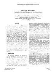
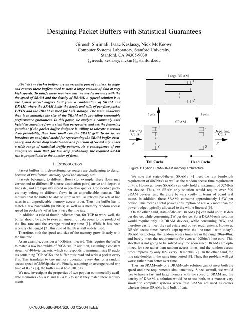
Figure 1: Hybrid SRAM-DRAM memory architecture.
Departing
Cells
We note that state-of-the-art SRAMs [4] meet the raw bandwidth
requirement of 80Gbits/s as well as the random access time requirement
of 4ns. However, these SRAMs can only hold a maximum of 32Mbits
per device. Thus, an SRAM-only solution would require over 300
SRAM devices, and therefore be very costly in terms of board real
estate. In addition, these SRAMs consume approximately 1.6W per
device. This means a total power consumption of 480W - more than the
power budget typically allocated to the whole linecard [6].
On the other hand, state-of-the-art DRAMs [5] can hold up to 1Gbits
per device, while consuming 2W per device. So, a DRAM-only solution
would require only 10 DRAM devices, while consuming 20W, and
therefore easily meet the real estate and power requirements. However,
DRAM access times haven’t kept up with the line rates - with today’s
DRAM technology, the random access times are in the range 20ns-40ns,
and barely meet the requirements for even a 10Gbits/s line card. This
shortfall is not going to be solved anytime soon since DRAMs are optimized
for size rather than random access times, and the random access
times improve by only 10% every 18 months [7]. On the other hand, the
line rate doubles in the same time period [8]. Thus, this problem will get
worse rather than better over time.
Thus, an SRAM-only or a DRAM-only solution cannot meet both the
speed and size requirements simultaneously. Since, overall, we would
like to have a fast and large memory with the speed of SRAM and the
density of DRAM, a solution would be to use both, in a manner very
similar to computer systems where fast SRAMs are used as caches
whereas dense DRAMs hold bulk of data.
1
Q
b cells
1
Q
R
0-7803-8686-8/04/$20.00 ©2004 IEEE

A common approach is to use a hybrid SRAM-DRAM architecture
[9][10][11], as shown in Figure 1. We encourage the reader to read [9]
for a detailed background and motivation for this architecture. Under
this architecture, one can envision the memory hierarchy as a large
DRAM containing a set of cell FIFOs with the heads and tails of
FIFOs in a dynamically shared SRAM.
The SRAM behaves like a cache, holding packets temporarily
when they first arrive and just prior to their departure. Variable size
packets arrive at the SRAM at rate R. They are segmented into fixedsize
cells and are stored into one of the Q tail FIFOs depending on
their flow ID. Later, a Memory Management Algorithm (MMA)
writes cells into the DRAM in blocks of b cells. Similarly, the MMA
transfers blocks of b cells from the DRAM FIFOs to the corresponding
head FIFOs in the SRAM. Finally, cells from head FIFOs depart
when requested by an external arbiter. Note that the MMA always
transfers b cells at a time - never less - between an SRAM FIFO and
the corresponding DRAM FIFO. By transferring b cells every b timeslots,
it ensures that the DRAM meets the memory speed requirement
in the long run. 1
In this paper, we look at the problem of independently sizing the
tail and head SRAMs from a statistical perspective under a wide range
of arrival traffic patterns. We provide models of the SRAM buffers,
present MMAs that would minimize the SRAM sizes for a given drop
probability, and derive formulas relating SRAM sizes to the drop
probability. As a consequence of our analysis we show that, in order
to provide low drop probability, the required SRAM sizes scales linearly
with Q . When Q is large, this linear dependence would make
such a buffer hard to implement. 2 Therefore, we exhibit an inherent
limitation of this architecture.
The rest of the paper is organized as follows. Section II presents a
model of the tail SRAM followed by a detailed analysis. Similarly,
Section III presents a model of the head SRAM along with analytical
results. Section IV provides some simulation results and Section V
concludes the paper.
A. Tail SRAM Model
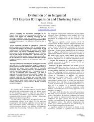
II. ANALYSIS OF THE TAIL SRAM
In this section, we introduce a queueing model for the tail SRAM,
together with some simplifying assumptions.
As illustrated in Figure 2, we model the tail SRAM as a single
queue served by a deterministic server of rate 1. For simplicity, we
assume time to be a continuous variable. A similar analysis could be
carried out in discrete time domain as well. We also assume that the
SRAM is dynamically shared among Q queues corresponding to Q
flows.
We denote by A( t)
the cumulative number of cells arriving at the
SRAM in [ 0,
t] . A( t) is assumed to be the sum of Q arrival processes
A i ( t) corresponding to the Q flows; A i ( t) have rates λ i such
that λ ≡∑1
λ . 3 i < We also assume that A i ( t)
are independent and
identically distributed (IID) stationary and ergodic processes. 4 We
similarly denote by D( t)
the cumulative number of departures in
1.
With line rate R, DRAM random access time T, and cell size c, we
define b = 2RT ⁄ c . Thus, T = b time-slots.
2. For example, in edge routers Q can be as large as a million.
3.
In this paper, all the finite sums are over index i over the range 1 to Q.
source 1
A 1 (t)
A Q (t)
source Q
A(t)
Figure 2: The tail SRAM model
+
[ 0,
t] . We then denote L( i,
t)
as the number of cells present in queue
i , and L( t) = L( i,
t)
as the total SRAM occupancy at time t.
To find the drop probability, we start by assuming that the SRAM is
infinite. We then obtain the steady state probability that the sum of
queue sizes exceeds S (i.e., P( L > S)
) as a surrogate for the steady
state overflow probability for an SRAM of size S .
We assume that the MMA works as follows [9]. Whenever the
DRAM is free, it serves an arbitrary queue from the set of all queues i
satisfying L( i,
t) ≥ b . For example, it could service the longest queue
with at least b cells, or the oldest queue with at least b cells, and so on.
We refer to this MMA as a b-Work Conserving MMA (BWC-
MMA) since it is work conserving as soon as at least one queue has
occupancy of at least . Because of work conservation, BWC-MMA
minimizes the tail SRAM occupancy among all possible MMAs in
this architecture. Therefore, given a tail SRAM of size S in the hybrid
architecture, BWC-MMA ensures that the drop probability P is minimized.
Equivalently, it minimizes S given a fixed P.
Under BWC-MMA, service to an individual queue depends on the
occupancy of all the queues in the system. Therefore, the queues are
not independent. For example, in one queue is being served, no other
queue
∑
b
can be served at the same time. This makes it hard to analyze
the queues in isolation, and we need to analyze the queue occupancies
together. This analysis is extremely challenging due to the interactions
between the queue occupancies.
B. The Fixed-Batch Decomposition
L(t)
D(t)
In this section, we simplify the analysis by decomposing the sum of
occupancies into elements that can be analyzed independently.
We start by noting that each A i ( t)
can be written down as
A i ( t) = b × MA i ( t)
+ R i ( t)
, (1)
where MA i ( t) and R i ( t)
are the quotient and the remainder after
A i ( t) is divided by b . Now the arrival process A( t)
can be written as
A( t) = A i ( t)
= ∑[ × MA i ( t)
+ R i ( t ) ] . (2)
We can also write
A( t) = b × MA( t)
+ R( t)
, (3)
where MA( t) = MA i ( t)
and R( t) = R i ( t)
are referred to as
the batch arrival process and remainder workload, respectively.
Having defined the arrival process, we now examine the departure
process. Since cells are serviced by fixed batches of b,
4. We believe this independence assumption is reasonable since the traffic
on a high speed WAN link usually comprises of traffic generated by
thousands of independent sources. In addition, in [12] we show that the
drop probability in the IID case upper bounds the corresponding probability
in the non-IID (independent but not identically distributed) case.
Thus, analysis for the IID case suffices for the scope of this paper.
∑
b

D( t) = b × MD( t)
, (4)
where MD( t)
represents the cumulative number of batch departures
in [ 0,
t]
.
Finally, having considered arrivals and departures, we look at the
sum of occupancies L( t)
, which can simply be written down as
L( t) = A( t) – D( t)
. (5)
Substituting for A( t) and D( t)
from Equation (3) and
Equation (4), we get
L( t) = [ b × MA( t)
+ R( t)
] – b × MD( t ) (6)
or
L( t) = b × ML( t)
+ R( t)
, (7)
where ML( t ) = MA( t) – MD( t)
is referred to as the batch workload.
Equation (7) indicates that the system workload L( t)
can be
decomposed into two terms. The first term, b × ML( t)
, is the product
of the batch size and the batch workload. The second term, R( t)
, is
simply the remainder workload.
We now show that the two terms in this decomposition are independent.
This greatly simplifies the analysis since it is now possible to
study them separately. The independence between the batch workload
and the remainder workload is provided by the following theorem.
Theorem 1: The remainder workload is independent of the batch
workload.
Proof: See
Theorem 1 provides what we call the fixed-batch decomposition. It
indicates that the steady state distribution of the system workload can
be derived simply by convolving the steady state distributions of the
remainder and batch workloads, i.e,
Appendix.
f L ( x) = f R ( x) ⊗ f ML ( x ⁄ b , )
(8)
where f L ( x) , f R ( x) , and f ML ( x)
are the steady state probability density
functions (PDF) of system, remainder, and batch workloads,
respectively. Thus, Theorem 1 allows us to translate the general queue
analysis to two more tractable problems.
C. Steady State Distributions
We first derive the steady-state distributions of remainder and batch
workloads. The fixed-batch decomposition can then be used to obtain
the steady-state distribution of the queue occupancy.
1) Steady State Distribution of the Remainder Workload
The steady state distribution of the remainder workload can be
given by the following theorem.
Theorem 2: As the number of flows increases (i.e., Q → ∞ ), the
steady state distribution of the remainder workload tends towards a
Gaussian distribution with mean Q( b – 1) ⁄ 2 and variance
Q( b 2 – 1) ⁄ 12 .
Proof: Appendix.
See
2) Steady State Distribution of the Batch Workload
Having derived the steady state distribution of the remainder workload,
we now derive the steady state distribution of the batch workload.
We use the batch queue model shown in Figure 3. In this model,
we analyze arrivals and departures of batches of cells instead of individual
cells. The batch arrival process is the superposition of Q IID
source 1
MA 1 (t)
MA Q (t)
source Q
MA(t)
Figure 3: The batch queue model
+
ML(t)
processes MA i ( t) , with total rate λ ⁄ b . Under the BWC-MMA discipline,
the batch queue is serviced by a work-conserving server of rate
1 ⁄ b .
Using Lindley’s recursion [13], the batch workload can be written
as
ML( t) = max 0 ≤ s ≤ t (( MA( t) – MA( s)
)–( t – s) ⁄ b)
. (9)
Equation (9) indicates that, given the steady-state distribution of
the batch arrivals, it is theoretically possible to derive the steady-state
distribution of the batch workload.
For general arrival patterns it is often not easy to find a closed-form
solution. However, for a broad range of arrival traffic patterns, the
superposition of an increasing number of flows can be shown to result
in a steady-state workload distribution that converges towards the
steady-state workload distribution of an M/D/1 queue.
To do so, we first make the following additional assumptions on the
arrival processes A i ( t) . We assume that each A i ( t)
is a simple point
process satisfying the following properties [14]. First, the expected
value of A i ( t) is given by λ i t . Second, a source cannot send more
than one cell at a time. And third, the probability of many cells arriving
in an arbitrarily small interval [ 0,
t] decays fast as t → 0 .
These assumptions are fairly general and apply to a variety of traffic
sources, including Poisson, Gamma, Weibull, Inverse Weibull,
ExpOn-ExpOff, and ParetoOn-ExpOff. These point processes model
a wide range of observed traffic [14], including wide area network
traffic.
Given these assumptions, we can state the following theorem.
Theorem 3: As the number of flows increases (i.e., Q → ∞ ), the
steady state exceedence probability P( ML > x)
of the batch workload
approaches the corresponding exceedence probability with a
Poisson source with the same load.
Proof: See
Theorem 3 shows that as the number of multiplexed IID sources
increases, the exceedence probability approaches the corresponding
probability assuming Poisson sources, which is known explicitly
through the analysis of the resulting M ⁄ D ⁄ 1 system
Appendix.
[15].
3) Steady State Distribution of the System Workload
MD(t)
Using the fixed-batch decomposition, f L ( x)
can easily be derived
as the convolution of f R ( x) and f ML ( x)
, which were obtained above.
We now provide an intuitive analysis of f L ( x)
for a large number
of flows. 5 For low values of λ , f ML ( x)
behaves like an impulse close
to zero. Since a convolution with an impulse at zero produces an output
equal to the input, f L ( x) would very much resemble f R ( x)
for
low values of λ , and therefore be close to a Gaussian.
5. In practice, we start observing the convergence indicated in Theorem 2
and Theorem 3 when the number of flows exceeds 100.

DRAM
L(t)
A(t)
SRAM
Buffer
F
I
F
O
MA ˆ
MD ˆ
( t)
( t)
D(t-LA)
Lookahead Buffer
D(t)
D(t-LA)
LA
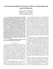
Figure 4: Theoretical PDF of L(t) for various loads for Q=1024 and
b=4 (the mean of the Gaussian is 1536)
Figure 4 plots f R ( x) and f L ( x)
as predicted by the theoretical
model and shows that this is indeed the case. At λ = 0.1 , the plots
corresponding to f R ( x) and f L ( x) are indistinguishable. At λ = 0.5 ,
the plots are still very close. The plots then separate out as the load
increases.
The main consequence of this observation is that, even for low
loads, f L ( x)
would result in more than 50% drops for an SRAM size
less than Q( b – 1) ⁄ 2 , the mean of the Gaussian. However, f L ( x)
falls very quickly due to the low variance of the Gaussian, and low
drop probabilities can be obtained close to Q( b – 1) ⁄ 2 . Therefore, to
give reasonable performance guarantees, the SRAM has to be slightly
more than Q( b – 1) ⁄ 2 , or Θ( Qb)
.
A. Head SRAM Model
III. ANALYSIS OF THE HEAD SRAM
As was the case for the tail SRAM, we assume the head SRAM to
be dynamically shared among Q flow queues. However, similarities
with the tail SRAM end here. For dynamic sharing to be useful for the
head SRAM, we need to be able to predict the (external) arbiter
request pattern in some way - if we can’t predict the request pattern to
the SRAM, we have to buffer up cells for each queue in a static way
and the advantage of dynamic sharing is lost. Thus, we assume the
presence of a fixed length lookahead buffer, which we use to predict
the request pattern to the SRAM. 6 Note that this assumes that the arbiter
is willing to tolerate a fixed delay LA between the arrival of
requests and the delivery of cells from the SRAM.
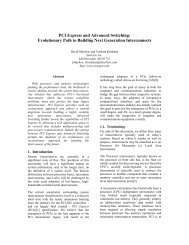
We use the scheme shown in Figure 5. Incoming requests ( D( t)
)
from an external arbiter enter the lookahead buffer to the right and
exit to the left after a fixed delay LA . Based on the requests in the
lookahead buffer and the cells in the SRAM, read requests ( MDˆ
( t)
)
are made to the DRAM so as to ensure that the cells ( A( t)
) are written
to the SRAM before the requests exit the lookahead buffer and
cells are read from the SRAM.
Similar to Section II.A, we define L( i,
t)
as the number of cells
present in queue i , and L( t) = L( i,
t)
as the total SRAM occupancy
at time t. We then define LR( i,
t)
to be the number of requests
for queue i in the lookahead buffer, and DEF( i,
t)
to be the deficit
∑
6.
This is inspired by the lookahead scheme in [9].
(number of arbiter requests for which a DRAM request has not been
made) for queue i at time t . A queue is defined to be critical at time
t if DEF( i,
t) < 0 .
We assume that the MMA works as follows [9]. Starting from an
empty SRAM, whenever the DRAM is free, it serves the earliest critical
queue from the set of critical queues, provided there is space in the
SRAM. If there are no critical queues then it doesn’t do anything.
In reference to Figure 5, the MMA operation can be described as
follows. When an arbiter request arrives, the deficit of the corresponding
queue is calculated. If the queue has gone critical, a read request is
is queued at the fetch FIFO, which is served in batches of b cells at
rate 1 ⁄ b . We now define FD( t)
to be the delay through the fetch
FIFO.
We refer to this MMA as a Deficit Work Conserving MMA (DWC-
MMA) since it is work conserving as soon as at least one queue has
gone critical. Because of the work conservation, DWC-MMA minimizes
the head SRAM occupancy among all possible MMAs in this
architecture. Therefore, given a head SRAM of size S in the hybrid
architecture, DWC-MMA ensures that the drop probability P is minimized.
Equivalently, it minimizes S given a fixed P.
In what follows we relate the (request) drop probability from the
head SRAM to the size of the lookahead buffer ( LA ) as well as the
size of the SRAM ( S ). This analysis can be extremely challenging
due to the interactions between the lookahead buffer and the SRAM.
B. Analysis of Head SRAM
The analysis of this complex system can be simplified as follows.
Observe that a request may not be served (or dropped) due to two reasons.
First, the lookahead buffer may not be deep enough to bring in
the required cells into the SRAM by the time the request traverses to
the end of the lookahead buffer. Second, even if the lookahead buffer
is deep enough, the SRAM may not be big enough to store the incoming
cells from the DRAM.
We refer to the overflowing of the lookahead buffer and head
SRAMs as events E1 and E2 , respectively. Now, the (request) drop
probability from the head SRAM of size S , using a lookahead buffer
of size LA , can be given by the following
P( S,
LA) = P( E1 ∪ E2)
, (10)
or
Figure 5: The head SRAM buffer model
P( S,
LA) ≤ P( E1) + P( E2)
. (11)

We again assume infinite buffers and use P( FD > LA)
and
P( L > S) as surrogates for P( E1) and P( E2)
, respectively. This lets
us rewrite Equation (11) as
P( S,
LA) ≤ P( FD > LA) + P( L > S)
. (12)
Thus, we can analyze P( FD > LA) and P( L > S)
separately to get
an upper bound on the drop probability of the head SRAM. It turns
out that both of these can be analyzed in a way very similar to the tail
SRAM.
C. A Model of the Queue
∑ ∑
Similar to Section II we can develop a model for the head SRAM
that is easy to analyze. We denote the request arrival process to the
SRAM by D( t) , where D( t)
is the cumulative number of requests
arriving in [ 0,
t] . D( t)
is further assumed to be generated by the
superposition of Q arrival processes D i ( t) , where D i ( t)
is the
cumulative number of requests sent for flow i in [ 0,
t] . Each D i ( t)
is assumed to have rate λ i , with
∑λ λ i = < 1 . In addition, we
assume that the request arrival processes D i ( t)
satisfy the assumptions
stated the cell arrival processes A i ( t)
in Section II.
We start by noting that each D i ( t)
can be written down as the following
D i ( t) = b × MD i ( t)
+ R i ( t)
, (13)
where R i ( t) and MD i ( t) are the remainder and quotient after D i ( t)
is divided by b .
Now, similar to Equation (3), the multiplexed process D( t)
can be
written as
D( t) = b × MD( t)
+ R( t)
, (14)
where MD( t) = MD i ( t)
and R( t) = R i ( t)
.
We now define a derivative process that is more useful in analyzing
the DRAM traffic due to DWC-MMA. The derivative process is
defined as ˆ
D i ( t) = D i ( t) + ( b – 1)
, (15)
which gives
Dˆ
( t) = D( t) + Q( b – 1)
. (16)
Now, breaking Dˆ i ( t) down in the same way as D i ( t)
, we get
Dˆ i ( t) = b × MDˆ i ( t)
+ Rˆ i ( t)
, (17)
where Rˆ i ( t) and MDˆ i ( t) are the remainder and quotient after Dˆ i ( t)
is divided by b . Thus, in a way similar to Equation (14), we get
Dˆ
( t) = b × MDˆ
( t)
+ Rˆ ( t)
, (18)
where MDˆ
( t) = MDˆ i ( t)
and Rˆ ( t) = Rˆ i ( t)
.
. MDˆ
( t)
is precisely the arrival process to the fetch FIFO. This is
due to the fact that, starting from an empty SRAM buffer, arrival
numbering 1,
b + 1,
2b + 1 , … to an SRAM queue result in fetches
from the DRAM.
Now, as mentioned earlier, the fetch FIFO is served at a rate 1 ⁄ b ,
resulting in the departure process MÂ( t) , where MÂ( t)
is related
to the arrival process to the SRAM buffer (i.e. A( t)
) in the following
way
A( t) = b × MA( t)
= b × MÂ( t – b)
. (19)
The first equality in Equation (19) represents the fact that arrivals
to the SRAM always occur in batches of b . The second equality
reflects the fact that
∑ ∑
the there is a fixed delay of b in reading from the
DRAM. Now, noting that the departure process from the SRAM
buffer is given by D( t – LA) , the SRAM buffer occupancy L( t)
can
be given by
L( t) = A( t) – D( t – LA)
. (20)
Using Equation (16) and Equation (19), we can write this as
L( t) = b × MÂ( t – b)
– ( Dˆ
( t – LA) – Q( b – 1)
) . (21)
Substituting for Dˆ
( t)
from Equation (18), we get
L( t) = b × ( MÂ( t – b) – MDˆ
( t – LA)
) + ( Q( b – 1) – Rˆ ( t – LA)
)
(22)
or
L( t) = b × ML( t)
+ RL( t)
, (23)
where
ML( t) = MÂ( t – b) – MDˆ
( t – LA)
(24)
and
RL( t) = Q( b – 1) – Rˆ ( t – LA)
. (25)
Realize that Equation (23) looks strikingly similar to Equation (7) -
in what follows, we show that it can be analyzed in a similar way.
However, for the sake of brevity, we intentionally stay away from
proving theorems that pretty much resemble the ones proved in Section
II, and state the results in an intuitive way.
We start by looking at the steady state distribution of RL( t)
(i.e,
f RL ( x) ). We note that f RL ( x)
can be obtained from the distribution of
Rˆ ( t) (i.e., f Rˆ ( x) ) by first flipping f Rˆ ( x)
around the origin and then
shifting to the right by Q( b – 1)
. 7 In addition, it can be proven, in a
way very similar to Theorem 2, that f Rˆ ( x)
is Gaussian with mean
Q( b – 1) ⁄ 2 and variance Q( b 2 – 1) ⁄ 12 . 8 So, for large Q , after
going through the linear transformations mentioned above, f RL ( x)
would pretty much be the same Gaussian as f Rˆ ( x)
.
Now we are ready to look at the distribution of ML( t)
. To do so,
we use the following inequalities
MDˆ
( t) – LA ⁄ b ≤ MDˆ
( t – LA) ≤ MDˆ
( t)
(26)
and
MÂ( t) – 1 ≤ MÂ( t – b) ≤ MÂ( t)
. (27)
In Equation (26), the right hand side inequality is pretty straightforward.
The left hand side inequality comes from the fact that in time
LA there can be at most LA ⁄ b fetch requests. Equation (27) can be
explained in a similar way.
Using Equation (26) and Equation (27) in Equation (24), we get
ML( t) ≤ MÂ( t) – ( MDˆ
( t) – LA ⁄ b)
(28)
or
ML( t) ≤ LA ⁄ b – ( MDˆ
( t) – MÂ( t)
)
(29)
or
ML( t ) ≤ LA ⁄ b – MLˆ ( t)
(30)
where MLˆ ( t) = MDˆ
( t) – MÂ( t)
is the occupancy of the fetch
FIFO. Equation (30) shows that the steady state distribution of
ML( t) (i.e., f ML ( x)
) can be obtained from the distribution of
MLˆ ( t) (i.e., f MLˆ ( x) ) by first flipping f MLˆ ( x)
around the origin and
then shifting to the right by LA ⁄ b . Note that, for IID D i ( t)
, Theorem
3 applies, and f MLˆ ( x)
can be derived as the steady state distribution
of an M ⁄ D ⁄ 1 queue.
At this point, we have the distributions of both the components of
Equation (23). It can be shown, in a way very similar to Theorem 1,
that Rˆ ( t) and MLˆ ( t)
are independent of each other, given the
assumptions on D i ( t) . Since RL( t) and ML( t)
are linear transformations
of Rˆ ( t) and MLˆ ( t)
, they are also independent of each other,
and the PDF of L( t) (i.e., f L ( x)
) can be obtained by convolving
f RL ( x) and f ML ( x)
, i.e.,
f L ( x) = f RL ( x) ⊗ f ML ( x ⁄ b)
. (31)
7. The steady state distribution of Rˆ ( t – LA)
is the same as the steady
state distribution of Rˆ ( t) as t → ∞
8.
While keeping similar assumptions in mind.

(a) load=0.5
Figure 6: Theoretical PDF of L(t) for various loads for Q=1024 and
b=4, with T=100*load
By analyzing for the distribution of L( t)
we can get one of the
quantities (i.e., P( L > S)
) required by Equation (12). To derive the
other quantity (i.e., P( FD > LA)
) we simply note that the delay
through the constant-service-rate fetch FIFO is directly related to the
occupancy of the FIFO, i.e.,
P( FD > LA) = P( MLˆ
> LA ⁄ b)
. (32)
Thus, by solving for the distributions of RLˆ ( t) and MLˆ ( t)
, we
get both the quantities required by Equation (12).
D. Putting it Together
We have talked about the sizes of the lookahead and SRAM buffers
as independent parameters. However, to get a reasonable value for the
upper bound indicated by Equation (12), we would have to first
choose a value of LA such that P( FD > LA)
is fairly low. Once we
have picked LA , we can then get P( L > S) using LA as a constant.
Note that this value of LA would depend only on the load λ . However,
in the M ⁄ D ⁄ 1 context, the value of LA to achieve low values
of P( FD > LA) may blow up in the limit λ → 1 . So, how do we
choose a value of LA that works for all traffic loads? The solution is
to limit the maximum load and assume that a design has a small speed
up - for example, a maximum λ of 0.9 would require a speed up of
1 ⁄ 0.9 ≅ 1.1 . Now, LA can be chosen for this maximum λ . In fact,
for large Q, the value of LA required to achieve low values of
P( FD > LA) turns out to be much smaller than Q( b – 1) ⁄ 2 .
Figure 6 plots f L ( x)
, as predicted by the theoretical model, for various
values of λ when Q = 1024 , b = 4 , and LA = cλ . We
picked c = 100 by noting that, as long as λ ≤ 0.9 , the steady state
distribution for the M ⁄ D ⁄ 1 queue dies out by the time the queue
occupancy gets to 100λ .
These plots are very similar to the ones in Figure 4, except for a
right shift by LA = cλ . For low values of λ , f ML ( x)
behaves like
an impulse close to LA ⁄ b . Thus, we expect f L ( x)
to very much
resemble a Gaussian centered about Q( b – 1) ⁄ 2 + LA . This would
of course change as λ → 1 , with the Gaussian being shifted to the
right and spread out a little. Again, note that in order to provide reasonable
performance guarantees, the head SRAM is required to be
Θ( Qb)
.
(b) load=0.9
Figure 7: Complementary CDF for b=4 and Q=1024
IV. SIMULATIONS
In this section we present some simulation results for the tail
SRAM and compare them to the predictions from Section II. The simulation
results for the head SRAM are similar, and are not presented
here.
Figure 7 plots of the drop probability as a function of the tail
SRAM size when b = 4 and Q = 1024 . These zoomed-out plots
correspond to the prediction from theory and simulation results for
two traffic types: Bernoulli IID Uniform and Bursty Uniform (the
burst lengths are geometrically distributed with average burst length
12).
We observe that the plots for λ = 0.5 are pretty much indistinguishable.
In addition, we observe that the plots are very close to the
Gaussian predicted by Theorem 2. Similarly, the plots for λ = 0.9
are very close to each other, with the plot from theory upper bounding
the other two for large values of queue occupancy. This shows the
power of Theorem 3 and indicates that the Poisson limit has already
been reached for Q = 1024 .
V. CONCLUSIONS
In this paper we presented a model for providing statistical guarantees
for a hybrid SRAM-DRAM architecture. We used this model to
establish exact bounds relating the drop probability to the SRAM size.
This model may be useful beyond the scope of this paper because it
may apply to many queueing systems with fixed batch service. These
systems are increasingly common due to the growing line rates and
the resulting use of parallelism and load-balancing.
Comparing to the deterministic, worst case analysis in [9], which
established Q( b – 1)
as the lower bound on SRAM size, we note that
our results provide an improvement by at most a factor of two. How-

ever, similar to [9], our bounds have a linear dependence on Qb . The
linear dependence on Q could be undesirable in cases where Q is
large.
Thus, our results can also be interpreted as an negative result for
this architecture. This can be stated in the following way: under the
hybrid SRAM-DRAM architecture, Θ( Qb)
is a hard lower bound on
the size of the SRAM, which can not be improved upon under any
realistic traffic pattern.
We believe this to be a characteristic of this architecture - since we
always transfer blocks of b cells, this results in storing Θ( b)
cells
for Θ( Q) flows, resulting in a total storage of Θ( Qb)
. This indicates
that we need to look at alternative architectures if design choices dictate
using SRAM sizes orders of magnitude lower than Θ( Qb)
.
REFERENCES
[1] C. Villamizar and C. Song, “High Performance TCP in ANSNET”,
Computer Communication Review, Vol. 24, No. 5, pp. 45--60, October
1994.
[2] G. Appenzeler, I. Keslassy, and N. McKeown, “Sizing Router Buffers”,
accepted at ACM SIGCOMM’04. Available at http://www.stanford.edu/~nickm.
[3] Caida, “Round-Trip Time Measurements from CAIDA’s Macroscopic
Internet Topology Monitor”, available at http://www.caida.org/analysis/performance/rtt/walrus0202/.
[4] Samsung, “Samsung K7N323645M NtSRAM”. Available at http://
www.samsung.com/Products/Semiconductor/SRAM/index.htm.
[5] Samsung, “Samsung K4S1G0632M SDRAM”. Available at http://
www.samsung.com/Products/Semiconductor/DRAM/index.htm.
[6] Cisco, “Cisco 12000 Series Two-Port OC-192c/STM-64c POS Line
card”. Available at http://www.cisco.com/en/US/products/hw/routers/
ps167/products_data_sheets_list.html.
[7] D. A. Patterson and J. L. Hennessy, Computer Architecture, A Quantitative
Approach, Section 8.4., pp. 425-432, Morgan Kaufmann, 1996,
[8] K.G. Coffman and A. M. Odlyzko, “Is there a “Moore’s Law” for data
traffic?,” Handbook of Massive Data Sets, eds., Kluwer, 2002, pp. 47-
93.
[9] S. Iyer, R. R. Compella, and N. McKeown, “Designing Buffers for
Router Line Cards”, Stanford University HPNG Technical Report -
TR02-HPNG-031001, Stanford, CA, 2002.
[10] S. Iyer, R. R. Kompella, and N. McKeown, “Analysis of a Memory Architecture
for Fast Packet Buffers,” IEEE HPSR’02, Dallas, Texas, May
2001.
[11] J. García, J. Corbal, L. Cerdà and M. Valero, “Design and Implementation
of High-Performance Memory Systems for Future Packet Buffers,”
Proceedings of the 36th Annual IEEE/ACM International Symposium
on Microarchitecture, p.373, 2003.
[12] G. Shrimali and N. McKeown, “Statistical Guarantees for Packet Buffers:
The Monolithic DRAM Case”, Stanford University HPNG Technical
Report - TR04-HPNG-020603, Stanford, CA, 2004.
[13] C.-S. Chang, Performance Guarantees in Communication Networks
London, Springer-Verlag, 2000.
[14] J. Cao and K. Ramanan, “A Poisson Limit for Buffer Overflow Probabilities”,
Proceedings of IEEE INFOCOM’02, pp. 994-1003, 2002.
[15] U. Mocci, J. Roberts, and J. Virtamo, Broadband Network Teletraffic:
Final Report of Action COST 242, Springer, Berlin, 1996.
. ∑ ∑
.
result.
For the first part, we start by proving that, for all i,j, R i ( t)
is independent
of MA j ( t) . For i ≠ j , R i ( t) is a function of A i ( t) , MA j ( t)
is
a function of A j ( t) , and A i ( t) is independent of A j ( t)
. Therefore
R i ( t) is independent of MA j ( t) . In addition, R i ( t) and MA j ( t)
are
independent of each other for i = j since A i ( t)
is stationary and
ergodic. Therefore, due to component-wise independence, the derived
processes MA( t) = MA i ( t)
and R( t) = R i ( t)
are independent
of each other. This finishes the first part of the proof.
Now, to prove the second part, we note that D( t) and MD( t)
are
functions of the process MA( t)
, and therefore are independent of
R( t) . Thus, ML( t ) = MA( t) – MD( t)
is also independent of
R( t)
Proof: (Theorem 2) The proof is in two steps. The first part involves
proving that the workload remainders R i ( t)
are IID. The second part
involves the application of the Central Limit Theorem.
For the first part, we note that R i ( t) depends only on A i ( t)
. Since
the parent processes A i ( t)
are independent of each other, the derived
processes R i ( t)
are independent of each other. Also, since the interarrival
times of arrival process A i ( t)
are stationary and ergodic,
R i ( t) would stay at each of the b states with equal probability, giving
P( R = x) = 1 ⁄ b,
∀x
. This is precisely the discrete uniform distribution,
Proof: (Theorem 3)We first show that if A i ( t)
are simple and stationary
point processes then MA i ( t)
are simple and stationary point processes.
Remember that each MA i ( t) is generated by taking every b th
sample of the corresponding parent process A i ( t)
. Therefore, in any
time interval, MA i ( t) will have fewer arrivals than A i ( t)
. So if
with mean ( b – 1) ⁄ 2 and variance ( b 2 – 1) ⁄ 12 .
Now, R( t) is a sum of Q IID uniformly-distributed random variables,
each with mean ( b – 1) ⁄ 2 and variance ( b 2 – 1) ⁄ 12 . By the
Central Limit Theorem, as Q → ∞ , R( t)
tends towards a Gaussian
random variable with mean Q( b – 1) ⁄ 2 and variance
Q( b 2 – 1) ⁄ 12
A i ( t)
satisfies properties of a simple point process (Section II.C.2),
then MA i ( t) will too. 9 Thus MA i ( t)
is a simple point process.
The stationarity of MA i ( t) follows from that fact that MA i ( t)
is
generated from A i ( t)
using a fixed sampling rule. Thus, if the characteristics
of the parent process A i ( t)
are stationary (i.e., independent
of time) then the characteristics of MA i ( t)
are stationary.
Thus, all the assumptions stated for A i ( t) are also true for MA i ( t)
.
This allows us to use Theorem 1 in [14] to get the required
APPENDIX
Proof: (Theorem 1) The proof is in two steps. The first part involves
proving the independence of R( t) and MA( t)
. The second part then
proves the independence of R( t) and ML( t ) .
9. Note that
E[ MA i ( t)
] = E[ A i ( t) ⁄ b] = λ i t ⁄ b