Evolutionary Algorithms Problem Set - MATLAB

Evolutionary Algorithms
Problem Set - MATLAB
General
This problem set contains MATLAB exercises to get you acquainted with the use of MATLAB
for Evolutionary Algorithms. The exercises are not mandatory, but are very useful for your
understanding of the subject matter, and in completing the practical assignment. If you have
questions or want to discuss your solutions, contact the teaching assistants.
1 Counting Ones
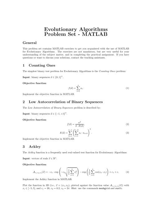
The simplest binary test problem for Evolutionary Algorithms is the Counting Ones problem:
Input: binary sequences ⃗a ∈ {0, 1} n .
Objective function:
f(⃗a) =
Implement the objective function in MATLAB.
2 Low Autocorrelation of Binary Sequences
The Low Autocorrelation of Binary Sequences problem is described by:
Input: binary sequences ⃗a ∈ {−1, +1} n .
Objective function:
n∑
a i . (1)
i=1
n2
f(⃗a) =
2 · E(⃗a) , (2)
(
n−1
∑ n−k
) 2
∑
E(⃗a) = a i · a i+k .
i=1
(3)
k=1
Implement the objective function in MATLAB.
3 Ackley
The Ackley function is a frequently used real-valued test function for Evolutionary Algorithms:
Input: vectors of reals ⃗x ∈ R n .
Objective function:
A c1,c 2,c 3
(⃗x) = −c 1 · exp
⎛
⎝−c 2
√ √√√
1
n
Implement the Ackley function in MATLAB.
n∑
i=1
x 2 i
⎞
⎠ − exp
(
1
n
)
n∑
cos(c 3 · x i ) + c 1 + e. (4)
Plot the function in 3D (i.e., ⃗x = (x 1 , x 2 ), plotted against the function value A c1,c 2,c 3
(⃗x)) with
x i ∈ [−5, 5], and c 1 = 20, c 2 = 0.2, c 3 = 2π. Hint: use the commands meshgrid and surfc.
i=1

4 Fletcher and Powell
The function after Fletcher and Powell, an example of a nonlinear parameter estimation problem,
is described by:
Input: vectors of reals ⃗x ∈ R n .
Objective function:
F A,B,⃗α (⃗x) =
p i (A, B, ⃗α) =
q i (A, B, ⃗x) =
n∑
(p i (A, B, ⃗α) − q i (A, B, ⃗x)) 2 , (5)
i=1
n∑
(a ij · sin(α j ) + b ij · cos(α j )) , (6)
j=1
n∑
(a ij · sin(x j ) + b ij · cos(x j )) , (7)
j=1
where A and B are n × n matrices (i.e., A and B contain n 2 elements a ij and b ij respectively)
and A, B, and ⃗α consist of random real values.
Implement this function in MATLAB, assuming A, B, ⃗α, and ⃗x are given as input.
5 Monte-Carlo Search for Binary Problems
Implement a Monte-Carlo Search algorithm (see slide 14 of lecture 1) for maximization problems
in MATLAB, in order to solve the Counting Ones problem. Let the function take the following
arguments:
• the objective function;
• the length n of the bitstrings ⃗a;
• the maximum number of fitness function evaluations.
Let the function produce as outputs:
• the best individual found by the algorithm;
• the fitness of the best individual.
Use n = 100 and for a run of 100 iterations, plot the fitness against the elapsed number of iterations.
Hint: store the current best solution found so far, and compare fitness value of new solutions
with this current best solution. Furthermore, you can pass a function as argument by putting the
@-symbol before the function name (i.e., it is passed as function handle).
6 Simple (1+1)-GA for Binary Problems
Implement the alternative method given in slide 18 of lecture 1 (this can be regarded as a simple
(1+1)-GA) for solving the Counting Ones problem, using the same approach as with the Monte-
Carlo Search algorithm of assignment 5.
Use n = 100 and a mutation rate p = 1/n. For a run of 100 iterations, plot the fitness against the
elapsed number of iterations. Is there a difference in performance compared to the Monte-Carlo
Search algorithm?

7 Monte-Carlo Search for Real-Valued Problems
Implement a Monte-Carlo Search algorithm for real-valued minimization problems in MATLAB.
Let the function take the following arguments:
• the objective function;
• the length n of the vector ⃗x;
• a vector of length n containing the lower bounds of the search domain;
• a vector of length n containing the upper bounds of the search domain;
• the maximum number of fitness function evaluations.
Let the function produce as outputs:
• the best individual found by the algorithm;
• the fitness of the best individual.
Run the algorithm on the Ackley function for 100 iterations with n = 2, x i ∈ [−5, 5], and c 1 = 20,
c 2 = 0.2, c 3 = 2π. Plot the fitness versus the number of iterations.
Note: we are now optimizing a minimization problem.
8 Simple (1+1)-EA for Real-Valued Problems
Think of a way of implementing the alternative method of assignment 6, now for dealing with
real-valued optimization problems.