Sample thesis 2 - Natural Computing Group, LIACS, Leiden University

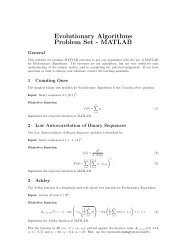
Squaring the CircleSeminar Swarm-based Intelligence – Fall 2010Johan de Ruiter, johan.de.ruiter@gmail.com(Project partner: Jelmer Cnossen)IntroductionThe topic of packing geometrical objects into a small volume is a very broad area of research whichhas a wide range of practical applications in industry and beyond. We chose to focus on aninteresting 2-dimensional packing problem that was first suggested by Erich Friedman of StetsonUniversity: Given a collection S n of squares with side lengths 1 to n, find the smallest possibleradius R n such that there exists a configuration of the squares in S n in the 2-dimensional plane, suchthat no squares overlap and all squares are contained within a circle with radius R n . Early resultswere due to Erich Friedman, Maurizio Morandi and the author [1].In this paper we highlight a number of interesting observations and algorithms that we derived fromscientific literature and we describe our findings stemming from our attempts to tackle the squarepacking problem by applying several different computing paradigms that were inspired by nature.Solution EvaluationBefore we can put any kind of optimizer to the test or compare our results with the best knownsolutions, we need a method to evaluate the quality of a solution. The question that arises is: Whatis the smallest circle enclosing a configuration of squares in the plane? But before we can evenattempt to answer this question, we should first ask ourselves how to check whether a given circle,determined by its center and its radius, does or does not enclose a given collection of squares in theplane. The answer to the latter question turns out to be fairly simple and quite elegant, but theunderlying principles are more intricate and making only slight modifications to the questionquickly demonstrates this.If one were to wave a square in front of a larger circle, one would notice that when moving thesquare from inside the circle to outside, one or more of the corners of the square will be the firstpoints to exit the circle. This hunch leads us to the correct assessment that a circle encloses a square(or a set of squares) if and only if it contains all of the corners of the square(s). However, if wewould ask ourselves whether a square is positioned completely outside the circle, it does not sufficeto merely check if all the corners are positioned outside the circle, for it is possible for a square toenter a circle with a point on its side first. Another possible modification would be to look at a ringrather than a circle, and then, depending on the size of the inner circle of the ring, it would bepossible for part of the inside of a square to be outside the ring, while its entire border is containedwithin the ring. Figure 1 serves to illustrate these concepts.The key concept at play here is convexity. Wikipedia states that “in Euclidean space, an object isconvex if for every pair of points within the object, every point on the straight line segment thatjoins them is also within the object” [2]. Now, a circle (or a disc rather, but we will stick with theterm circle) is convex and a square is convex. In fact, a square is the convex closure of its 4 corners,because the borders of the square are the straight line segments between pairs of these points, andfurthermore, every point inside the square is on the straight horizontal line between two points onthe square's border. As a consequence of the convexity of the circle and the square, if the corners ofa square are contained within a circle, then so is every other point in the square. Trivially, if theentire square is contained in the circle, then so are its corners. This proves our claim that a square iscontained within a circle if and only if its 4 corners are contained in it.

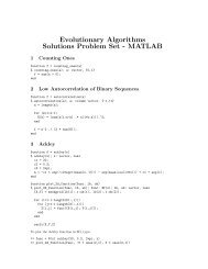
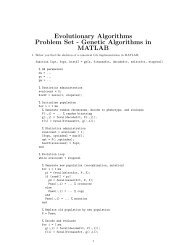
Figure 1: (a) The corners of a square are the first to appear outside of a circlewhen moving a square outward from within a circle. (b) The corners are notnecessarily the first to enter a circle when moving inward from outside a circle.(c) A square can have all its corners contained within a ring and still not becontained in it in its entirety.The Smallest Enclosing CircleNow we know how to judge whether or not a circle contains a collection of squares, we are ready toset out to find the smallest enclosing circle.The most straightforward algorithm exploits the following observations:1. Three distinct non-colinear points uniquely determine the circle going through them.2. Two distinct points uniquely determine the smallest circle going through them.To help build the intuition required, Figure 2 illustrates the smallest circle through two points andtwo instances of the unique circle through three non-colinear points.Figure 2: The smallest circle through two points (left) andinstances of circles uniquely determined by three non-colinearpoints (center and right).As a result of these observations it suffices to check for each of the O(n 2 +n 3 ) = O(n 3 ) (smallest)circles uniquely determined by either two or three points whether or not all O(n) points in the set arecontained within it. After all, if the smallest enclosing circle would not be going through two orthree points, we would be able to shrink it without leaving any points out, which would contradictthe fact that it was the smallest possible.Finding the center and the radius of the smallest circle going through a pair of points can be done inconstant time. We have to realize that the center of such a circle c is exactly in between the twopoints p 1 and p 2 . In formulas:c x =(p 1,x +p 2,x )/2c y =(p 1,y +p 2,y )/2c radius =sqrt((p 1,x -p 2,x ) 2 +(p 1,y -p 2,y ) 2 )/2Finding the center and the radius of the unique circle going through three points takes a bit more

work to figure out formula-wise, but once the math has been done, this can also be performed inO(1) time. We have to start by expressing the fact that the center of the circle c has the sameeuclidean distance to each of the three points p 1 , p 2 and p 3 in a set of equations:c radius2=(c x -p 1,x ) 2 +(c y -p 1,y ) 2 =(c x -p 2,x ) 2 +(c y -p 2,y ) 2 =(c x -p 3,x ) 2 +(c y -p 3,y ) 2Solving these equations for c x and c y respectively gives the expressions:c x =((p 1,y -p 2,y )(p 3,x2 +p 3,y2 )+(p 2,y -p 3,y )(p 1,x2 +p 1,y2 )+(p 3,y -p 1,y )(p 2,x2 +p 2,y2 ))/(2((p 1,y -p 2,y )p 3,x +(p 3,y -p 1,y )p 2,x +(p 2,y -p 3,y )p 1,x ))c y =((p 1,x -p 2,x )(p 3,x2 +p 3,y2 )+(p 2,x -p 3,x )(p 1,x2 +p 1,y2 )+(p 3,x -p 1,x )(p 2,x2 +p 2,y2 ))/(2((p 1,x -p 2,x )p 3,y +(p 3,x -p 1,x )p 2,y +(p 2,x -p 3,x )p 1,y ))To find the radius we don't have to find an expression in terms of only the coordinates of the threepoints; we can use the values we computed for c x and c y together with one of the earlier formulas:c radius =sqrt((c x -p 1,x ) 2 +(c y -p 1,y ) 2 )Checking whether a point p 4 lies within a circle of which one knows both the center and the radiusis done in O(1) by verifying whether (c x -p 4,x ) 2 +(c y -p 4,y ) 2

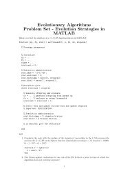
Figure 3: Without the need for manywords this image makes clear that thesmallest enclosing circle of a set ofpoints is uniquely determined [7].Uniqueness of the Smallest Enclosing CircleWe already kind of implicitly stated that the smallest enclosing circle of a set of points is uniquelydetermined, but we do so now explicitly in the context of Welzl's Algorithm. Figure 3, which wasborrowed from [7], illustrates the concept very well without the need for many words.We provide a proof by contradiction: Suppose that the smallest enclosing circle is not uniquelydetermined and that we have a collection of points which has distinct smallest enclosing circles D 1and D 2 (by definition of equal radius), then all of the points are contained within the area where D 1and D 2 overlap. However, as the green line in Figure 3 indicates, we can draw a circle of smallerradius through the points where D 1 and D 2 intersect. This contradicts the fact that D 1 and D 2 are thesmallest enclosing circles and we can therefore conclude that our assumption was wrong and thatthe smallest enclosing circle must be uniquely determined.A Useful LemmaAnother piece of information that we will rehash from the O(n 4 ) smallest enclosing circle algorithm,now comes in the form of a technical lemma that states: Given a set of points P, there is a subset Sof P with |S|

Figure 6: The best known solutions for 1 to 15 squares, by Erich Friedman (theones uncredited in the image), Maurizio Morandi and the author [1].

A Feasibility ProblemWhen we approach the problem of finding a configuration of a set of squares for which the smallestenclosing circle is minimal with an evolutionary strategy or a particle swarm, it makes sense to usethe radius of the smallest enclosing circle as the fitness value to minimize.The most obvious representation of a configuration of squares is a set of coordinates in some wayrepresenting the position of a square (for example the top left corner or the center). There is onemajor drawback to this choice: Because of overlapping squares many elements in the solution space 2n are infeasible. We came up with, and implemented, two different solutions:1) For each pair of squares that overlaps we add a penalty that is linear in the size of theirintersection. In case one square is completely contained within the other we give an extrapenalty related to the distance the squares need to travel to be separated. We felt it would benecessary to add an extra constant penalty for having any overlap at all, because it should beavoided that the optimizers will find solutions in which they trade a small overlap penaltyfor a significant decrease in radius.The problem of finding the overlap between two squares, or more generally, two rectanglesaligned to the same grid axes, can be reduced to finding the overlap of their projections onboth of the axes and multiplying their lengths. This reduces the problem to finding theoverlap of two intervals on a line, which is relatively easy to do.2) We map every configuration that does not have any identical coordinates for differentsquares to a feasible configuration in two steps (if there are happen to be identicalcoordinates then they can be changed with a minor mutation). First of all we shrink allsquares by the same ratio f, until no squares overlap anymore and at least one pair of squarestouches. The value of f can be computed in O(n 2 ) time by computing the shrinking ratio forevery pair of squares. Theoretically it seems this could also be done in O(n log n), if wewould compute the Delaunay triangulation [8], but this is quite clearly overkill. The secondstep in the process is to scale the configuration in its entirety such that the squares regaintheir original size. This would be done in linear time. Interestingly, the shrinking andrescaling operations can be combined, because of how we store the squares. First wecompute the ratio f, and then we simply divide all coordinates by f.Solution 2 also lends itself for fine-tuning feasible solutions before evaluating them, as the samemathematics can pack configurations in which no squares touch more tightly. We will work out anexample in detail to illustrate the fine-tuing rather than the removal of overlap, just because theimage will most likely be easier to understand.Figure 7: A configuration of twosquares before and after fine-tuning,modulo a translation and zoomed in.

Figure 7 shows a configuration of a pair of squares with sides s 1 =2 and s 2 =4 with their centers at(11, 5) and (5, 5) respectively. The vertical distance between their centers is ∆v=0, the horizontaldistance between their centers is ∆h=6 (as indicated by the black line). We are interested only in themaximum of these values, which happens to be 6. The ratio f=max(∆v,∆h)/(s 1 /2+s 2 /2)=2*max(∆v,∆h)/(s 1 +s 2 )=2*6/(2+4)=2. In the next step we divide the coordinates by f, resulting in(6.5, 2.5) and (2.5, 2.5), which correspond with the touching red squares in Figure 7, modulo atranslation and after zooming in by a factor 2 (the problem of the smallest enclosing circle isinvariant under translations of all squares by the same vector). When there are more than twosquares involved, we have to use the smallest value among the computed f's.However, although clever and mathematically elegant, method 2 turns out not not to work well inpractice with any optimizer we tried.Observations and Practical ConsiderationsWe wrote a number of optimizers to tackle the problem at hand and we experimented with manydifferent modifications to the standard algorithms. Because the problem inspired us to come up withso many different tweaks and adaptations to experiment with, and because the interactions betweenall these different tricks are often so fundamentally interrelated in ways that are mostly too complexto predict or even analyze, it was very difficult to choose sets of features to test with extensively,given a finite time. The stochastic nature of the experiments involved and the reasonably largenumber of parameters to set made it even more difficult, because it is not always easy to rankdifferent behaviors when short term behavior might not accurately represent the value of a certainapproach in the long run and when short term marginal differences might or might not carrysignificance. To add insult to injury, different choices might be beneficial for different instances ofthe problem: Something that works well when dealing with 5 squares might be disastrous whendealing with 15 squares, and vice versa.We will describe and discuss a number of tricks that we came up with and we will elaborate onobservations that we made over the course of the project.Particle Swarm Optimizer DiscardedWe first embarked on applying a canonical particle swarm optimizer to the problem [10]. This didnot bring us the results we had hoped for, not even after parameter tuning, and eventually we sawno other option than to abandon trail and switch to another kind of optimizer. The friendshiptopologies we experimented with are the fully connected graph K n , a star graph, a forest of disjointstar graphs, a 2-dimensional lattice grid graph and a cyclic graph.The problem seemed to be the fact that many parameters that were not immediately crucial for thequality of a configuration (for example, because they were located in the center by themselves,while other squares were spanning the circle), were quickly tending towards zero, leading to earlystagnation across the entire population. In the remainder of the text we will solely focus onevolutionary strategies (ES) [9].RepresentationsTo follow up on what we mentioned earlier, the most straightforward way of representing a solutionfor any optimizer is to have a vector v of 2n floating point numbers in which the elements v 2i-1 andv 2i for (1

At some point we decided to fix the largest square at location (0,0) to avoid repeatedly having totranslate our configurations back to some reliable reference location when they would drift off intoregions of 2n where the accuracy of the floating point implementation became questionable.A side-effect of fixing the largest square is a reduction of the state space by 2 dimensions. This gain,however, does not come without any strings attached: The largest square is now not free to move.Although still any configuration of squares can be represented (as they are invariant undertranslation), if some translation of this square or a swap with this square involved would bebeneficial, then the collection of all other squares would need to be adapted instead to attain thesame result. The probability that this would happen by itself is generally much lower than what wewould deem natural. This can be accepted as a drawback, or it can be dealt with pro-actively byimplementing an actual realization of these operations and applying them whenever appropriate, butthe option to implement these features is mildly annoying with the foresight that we will be addingmore complex operations in the future, often experimental, and which would ideally all come withthe appropriate functionality to make up for the static nature of the largest square.With all these things in mind, perhaps fixing the coordinates of a square might not have been thebest choice. However, we would like to argue that given that the choice was made to fix thecoordinates of a square and not provide said functionality, the largest square is at least a betterchoice than the smallest square. Two reasons are firstly the fact that when the largest square moves,on average it has a higher probability than others to overlap (given similar circumstances), andsecondly the special role we have in mind for the smallest square (described in the next paragraph).On the other hand, one might argue the contrary by stating that exactly because the smallest squarehas the lowest probability to overlap other squares (given similar circumstances), it being fixedwould hardly be noticed, especially for larger instances, and would therefore hardly disrupt thefitness landscape.Dimensionality ReductionAnother way to reduce the dimensionality of the problem is to remove the smaller squares,assuming they will fit anywhere and can be put somewhere in the end. We did not implement this ason the other hand small squares don't always have to be in the way and one of the adaptations wewill discuss particularly depends on their presence. The question which set of smaller squares canbe left out for a given number of squares is interesting and non-trivial.We thought it would be interesting to temporarily link touching squares to reduce the problemdimensionality and limit the number of overlaps, but we did not get to implement it.Dynamic Data StructuresA very refreshing idea in the setting of evolutionary strategies, in our opinion, would be to maintaina dynamic data structure with efficient update- and query operations to perform evaluations morequickly. A requirement would be that either the data structure is very lightweight and can be copiedand maintained faster than we can do regular fitness evaluations, or that we can somehow manageour resources such that we can avoid copying the entire data structure time and time again.Matousek [12], which is based on Megiddo's parametric search [13], seems to be a good startingpoint for a dynamic data structure revolving around the smallest enclosing circle problem.A Special Task SquareIt was foreshadowed above that the square with sides of length 1 could potentially fulfill a specialpurpose. For many squares, especially the larger ones, moving them around over larger distanceswould most often result in solutions of very low quality, because of the high probability of beingheavily penalized for overlapping. We could search for locations where a square could fit, if at any

sensible location at all, but it is not immediately obvious how to do that and how to do thatefficiently.We will exploit the fact that the smallest square will usually fit in many locations. Possible targetpositions are generated until one is found where this small square will actually fit. We implementedthe check in linear time, but we suspect theoretically it would be possible to do this faster if a kdtreeis maintained throughout [11]. That the use of such a datastructure would have any practicalsignificance for the numbers of squares we deal with remains doubtful.Preferably we would target only positions within or very near the smallest enclosing circle. The waywe chose to do it is to temporarily shift to polar coordinates. In polar coordinates a point isdescribed as a pair (angle theta, radius r). To get a uniform distribution over the circle we chosetheta to be uniformly distributed over [0,2π) and r to be 1 minus the square of a uniform randomvariable in [0,1], multiplied by an approximate radius of the smallest enclosing circle. The squaringhappens to compensate for the density function of the projection of the circle on the positive part ofthe radial line. We could invoke our evaluation function to find the center and the radius of thiscircle, but somehow it felt unnatural to us to waste evaluation functions, given that they areprobably slower than quick and dirty estimation methods (even if just by a constant) that couldwork about as well. We could for example take the leftmost, rightmost, uppermost and bottommostpoints, and base our estimate on those. Once again, a kd-tree might theoretically allow for fastermethods than linear time, but for practical purposes a linear sweep seems just fine.The real value of this special purpose of the smallest square comes to light when we combine theapproach described with the kind of mutation explained in the following paragraph.SwapsAn interesting observation to make is that swapping the midpoint coordinates of two squares thatare roughly the same size, in a part of the packing that is not too tight, can exploit previouslyunused paths between solutions of similar fitness through the fitness landscape without having to gothrough deep valleys that would be difficult to cross. We made the probability that a square wouldbe involved in such a mutation inversely proportional to the square of its side-lengths. Its swappartner would be decided by a random variable drawn from a normal distribution. The valuestandard deviation used eventually was 1.5.Some evidence suggests that the probability with which we involved larger squares in swaps wastoo high. This came to light when a bug lowering those odds was found to be a mysterious feature.It must be said that it is extremely difficult to assess how a thing like such a bug affects the balancebetween exploration and exploitation and the balance between sense and nonsense. As aconsequence it is very hard to restore the balance once the perceived disturbance has beencorrected.In combination with the strategy implemented for the smallest square, we see a very powerfulbehavioral pattern emerge: The smallest square continuously explores new territories and thepermitted swaps allow other squares that could fit there to follow in its footsteps. A drawback of thesuccess of this strategy might be that there is much less focus on the self adaptation, with lessevolutionary pressure on self adaptation leading to less benefit from it.We were faced with two options: Either we would swap the sigma values along with thecoordinates, meaning they are essentially tied to a location, or we would leave them untouched,meaning they are essentially tied to a square. We are convinced the latter makes much more sense,because the relationship between a location susceptible to a wide range of mutations and a variablefor self-adaptation seems much too volatile to be of any practical value.

We also considered to implement swaps between squares and their nearest neighbors (for someappropriate measure of distance). If we make such a swap, we know that afterwards these twosquares will not overlap each other if they did not do so beforehand, but the larger of the twosquares involved could overlap surrounding squares that the smaller of the two did not overlap inadvance of the swap. A fast implementation, at least theoretically, could (once again) be provided bya kd-tree. A possibly useful variation could be to facilitate swaps between squares near the edges ofthe smallest enclosing circle, possible preventing overlaps using translations. Neither nearestneighborswaps, nor edge-square swaps are incorporated in the project at this point.Yet another possibility is to compute for each square with which squares it could be swappedwithout causing overlaps. This could greatly reduce the number of wasted individuals.SeasoningInspired by simulated annealing [14] we experimented with what we branded seasoning. Theconcept comes in several different flavors and serves to spice up an evolutionary strategy. The mainingredient is a repeated time interval, a season, over which some quantity is varied according to acertain recipe.The rationale behind it is twofold. First of all, the very phenomenon simulated annealing wasmodeled after, annealing in metallurgy, which occurs by the diffusion of atoms within a solidmaterial [15], bears a striking resemblance to the square packing problem (but the fitness landscapeof the square packing problem shows much more variation). A recipe conceptually resembles thecooling schedule used in simulated annealing. Secondly, our problem is highly multimodal and wewould like to combine serious exploration with far reaching exploitation, but preferably notconcurrently. A good recipe is one that allocates ample time to each of these and arranges for aproper transition between different phases.The most basic recipe we used over the course of this project regulated the upper and lower boundson the sigma values by a sinusoidal wave. We also tried a recipe in which bounds on the sigmavalues were slowly decreasing while also lowering the rate of the other types of mutation. In thiscase we could abandon a season when by the time we arrived to the exploitation stage it was ratherclear that this attempt would not lead to the global optimum. Lastly, we also incorporated shortperiods of a gravitational force from the center of the to put everything together tightly. This will beexplained below.Exploration can encouraged when a dead end is reached, either by randomization or by increasingthe sigma values temporarily.Overlap Avoidance StrategyWe designed a computationally cheap but quite effective method to avoid overlaps because ofmoving squares. Four sets are maintained for each individual, containing the x-coordinates of theirleft sides, the x-coordinates of their right sides, the y-coordinates of their upper sides and the y-coordinates of their bottom sides respectively; each element is accompanied by its side length, butthe order on the set does not take the side lengths into account. Inserts and search queries onmultisets take logarithmic time. Erasures can be considered to take logarithmic time on averagegiven that squares are not expected to align themselves. Looking for the next higher value can bedone in constant time after a logarithmic time search query. In this way we can limit the movementof a square with a logarithmic time check, as the movements are typically small and number ofsquares that could be in the way is small as well, while we can test each of them for overlap inconstant time. In our implementation we simulated this behavior with a linear time algorithm, as forsmall instances this would most likely outperform the heavier costs of a heavier datastructure.

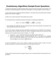
Notice that as long as this strategy is employed nearly all the exploration depends on swaps, whichmight not be the behavior desired.Gravitational ForceA gravitational force was an ingredient in some of our recipes. For a short period of timemovements towards the center of the smallest enclosing circle of the local optimum were favoredover others. However, one might wonder, how that can be done given that we don't know where thisoptimum is located? We believe the answer lies in favoring movements towards an expected centerwith a higher probability. The expected center can be based on extreme values maintained or by afitness evaluation.When we didn't fix the sigma values during such a period of gravitational force, while we were notusing the overlap avoidance strategy described, this period was observed to be followed by a periodof randomization because these were not as much subjected to selective pressure.Results and ConclusionsWe would like to stress that we started this project with the goal in mind to improve existing resultsfor 15 circles or less in the unlikely event that these were not optimal (at least up until a few digitsbehind the decimal point) and to find optimal rather than decent scores for slightly larger instancesof the problem. After all, only optimal solutions will carry the names of the discoverers indefinitely.Our research therefore mostly focused on finding the global optima, rather than on creatingalgorithms that perform reasonable in the average run.Summarizing the development process, there was a lot of tweaking of the code and many featureswere implemented and consequently tested, but we were never really satisfied. The absence of goodresults became quite frustrating in the end, because we wanted to run tests for longer time, but therewas always a reason to think that the next trick or attempt to fine tune would fix everything and itnever really did. For the same reason the circumstances under which the best found solutions wereacquired have not been well-documented; we didn't think they would forever remain the best foundsolutions, or we assumed that our final code would easily find them back.Figure 8: The best solution we found for 15squares had a smallest enclosing circle with aradius of 22.513, while the best known solutionhas a radius of 21.631.Figure 9: The best solution we found for 16squares had a smallest enclosing circle withradius 24.700.

As we are not satisfied with the current state of the code base, we feel it adds very little value toinclude a comparative analysis between different runs with different parameters. What we canreport is the following: Up until the amount of 11 squares we have at some point producedconfigurations with the same radius as the best known solutions. For 12 and 13 squares we have atsome point produced configurations that resembled the best known solutions, but we did not getmore than 2 digits behind the decimal point correct. An indication that something was wrong withour ability to zoom in on solutions. For 14 and 15 squares we have produced configurations thatwere good, but not optimal.Figure 8 shows the best solution found for 15 squares. Figure 9 shows the best solution we foundfor 16 squares, and it might or it might not be optimal. Our other results lead us to believe that itcould probably at the very least benefit from further fine tuning. After properly refining it we willreport the coordinates of this new discovery to Erich Friedman.Despite the disappointing results, we most certainly plan to get back to this problem in the future.Perhaps with a more mathematical approach, or with a canonical simulated annealingimplementation.

References[1] E. Friedman, Math Magic (July 2010),http://www2.stetson.edu/~efriedma/mathmagic/0710.html, retrieved December 2010.[2] Wikipedia – The Free Encyclopedia, Convex Sethttp://en.wikipedia.org/wiki/Convex_set, retrieved December 2010.[3] J. Elzinga and D.W. Hearn, The Minimum Covering Sphere Problem, Management Science,Vol. 19, 96–104, 1972.[4] M.I. Shamos and D. Hoey, Closest-point problems, focs, 151–162, 16th Annual Symposium onFoundations of Computer Science (FOCS 1975), 1975 .[5] N. Megiddo, Linear-Time Algorithms for Linear Programming in R3 and Related Problems,SIAM Journal on Computing, Vol. 12, 759–776, 1983.[6] E. Welzl, Smallest enclosing disks (balls and ellipsoids). In H. Maurer, editor, New Results andNew Trends in Computer Science, volume 555 of Lecture Notes Comput. Sci., 359–370, Springer-Verlag, 1991.[7] Sunshine, Computing the smallest enclosing disk in 2D, 2008,http://www.sunshine2k.de/stuff/Java/Welzl/Welzl.html, retrieved December 2010.[8] Wikipedia – The Free Encyclopedia, Delaunay triangulation,http://en.wikipedia.org/wiki/Delaunay_triangulation, retrieved December 2010.[9] T. Bäck, Evolutionary Algorithms in Theory and Practice: Evolution Strategies, EvolutionaryProgramming, Genetic Algorithms, Oxford Univ. Press, 1996.[10] J. Kennedy, R. Eberhart, Particle Swarm Optimization, Proceedings of IEEE InternationalConference on Neural networks IV, 1942–1948, 1995.[11] Wikipedia – The Free Encyclopedia, kd-tree,http://en.wikipedia.org/wiki/Kd-tree , retrieved December 2010.[12] J. Matousek, Linear optimization queries, J. Algorithms, 14, 432–448, 1993.[13] N. Megiddo, Applying Parallel Computation Algorithms in the Design of Serial Algorithms,Journal of the ACM (JACM), v. 30 n. 4, 852–865, 1983.[14] S. Kirkpatrick, C. D. Gelatt, M. P. Vecchi, Optimization by Simulated Annealing, Science, NewSeries 200, 671–680, 1983.[15] Wikipedia – The Free Encyclopedia, Annealing (metallurgy)http://en.wikipedia.org/wiki/Annealing_(metallurgy), retrieved December 2010.