Use of Rational and Modified Rational Method for ... - CTR Library
Use of Rational and Modified Rational Method for ... - CTR Library
Use of Rational and Modified Rational Method for ... - CTR Library

You also want an ePaper? Increase the reach of your titles
YUMPU automatically turns print PDFs into web optimized ePapers that Google loves.
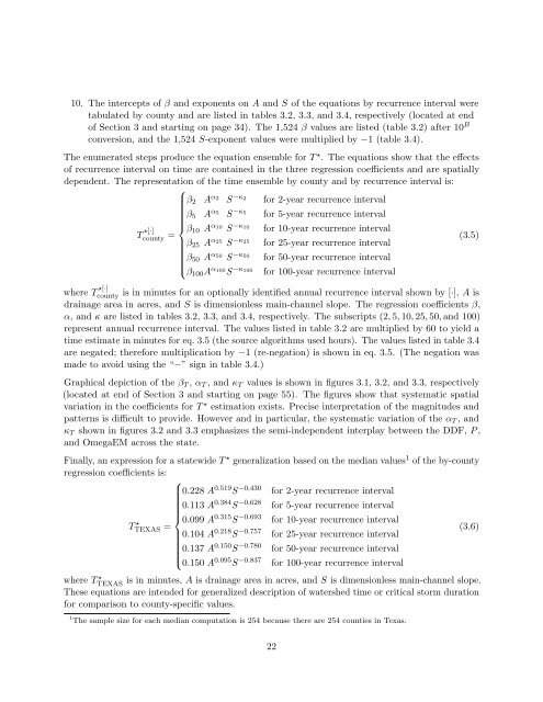
10. The intercepts <strong>of</strong> β <strong>and</strong> exponents on A <strong>and</strong> S <strong>of</strong> the equations by recurrence interval were<br />
tabulated by county <strong>and</strong> are listed in tables 3.2, 3.3, <strong>and</strong> 3.4, respectively (located at end<br />
<strong>of</strong> Section 3 <strong>and</strong> starting on page 34). The 1,524 β values are listed (table 3.2) after 10 B<br />
conversion, <strong>and</strong> the 1,524 S-exponent values were multiplied by −1 (table 3.4).<br />
The enumerated steps produce the equation ensemble <strong>for</strong> T ⋆ . The equations show that the effects<br />
<strong>of</strong> recurrence interval on time are contained in the three regression coefficients <strong>and</strong> are spatially<br />
dependent. The representation <strong>of</strong> the time ensemble by county <strong>and</strong> by recurrence interval is:<br />
β 2 A<br />
⎧⎪ α 2<br />
S −κ 2<br />
<strong>for</strong> 2-year recurrence interval<br />
β 5 A α 5<br />
S −κ 5<br />
<strong>for</strong> 5-year recurrence interval<br />
⎨<br />
county = β 10 A α 10<br />
S −κ 10<br />
<strong>for</strong> 10-year recurrence interval<br />
β 25 A α 25<br />
S −κ 25<br />
<strong>for</strong> 25-year recurrence interval<br />
⎪ ⎩<br />
T ⋆[·]<br />
β 50 A α 50<br />
S −κ 50<br />
<strong>for</strong> 50-year recurrence interval<br />
β 100 A α 100<br />
S −κ 100<br />
<strong>for</strong> 100-year recurrence interval<br />
(3.5)<br />
where T ⋆[·]<br />
county is in minutes <strong>for</strong> an optionally identified annual recurrence interval shown by [·], A is<br />
drainage area in acres, <strong>and</strong> S is dimensionless main-channel slope. The regression coefficients β,<br />
α, <strong>and</strong> κ are listed in tables 3.2, 3.3, <strong>and</strong> 3.4, respectively. The subscripts (2, 5, 10, 25, 50, <strong>and</strong> 100)<br />
represent annual recurrence interval. The values listed in table 3.2 are multiplied by 60 to yield a<br />
time estimate in minutes <strong>for</strong> eq. 3.5 (the source algorithms used hours). The values listed in table 3.4<br />
are negated; there<strong>for</strong>e multiplication by −1 (re-negation) is shown in eq. 3.5. (The negation was<br />
made to avoid using the “−” sign in table 3.4.)<br />
Graphical depiction <strong>of</strong> the β T , α T , <strong>and</strong> κ T values is shown in figures 3.1, 3.2, <strong>and</strong> 3.3, respectively<br />
(located at end <strong>of</strong> Section 3 <strong>and</strong> starting on page 55). The figures show that systematic spatial<br />
variation in the coefficients <strong>for</strong> T ⋆ estimation exists. Precise interpretation <strong>of</strong> the magnitudes <strong>and</strong><br />
patterns is difficult to provide. However <strong>and</strong> in particular, the systematic variation <strong>of</strong> the α T , <strong>and</strong><br />
κ T shown in figures 3.2 <strong>and</strong> 3.3 emphasizes the semi-independent interplay between the DDF, P ,<br />
<strong>and</strong> OmegaEM across the state.<br />
Finally, an expression <strong>for</strong> a statewide T ⋆ generalization based on the median values 1 <strong>of</strong> the by-county<br />
regression coefficients is:<br />
⎧<br />
0.228 A 0.519 S −0.430 <strong>for</strong> 2-year recurrence interval<br />
0.113 A 0.384 S −0.628 <strong>for</strong> 5-year recurrence interval<br />
⎪⎨<br />
TTEXAS ⋆ 0.099 A 0.315 S −0.693 <strong>for</strong> 10-year recurrence interval<br />
=<br />
0.104 A 0.218 S −0.757 <strong>for</strong> 25-year recurrence interval<br />
0.137 A 0.150 S −0.780 <strong>for</strong> 50-year recurrence interval<br />
⎪⎩<br />
0.150 A 0.095 S −0.837 <strong>for</strong> 100-year recurrence interval<br />
where TTEXAS ⋆ is in minutes, A is drainage area in acres, <strong>and</strong> S is dimensionless main-channel slope.<br />
These equations are intended <strong>for</strong> generalized description <strong>of</strong> watershed time or critical storm duration<br />
<strong>for</strong> comparison to county-specific values.<br />
1 The sample size <strong>for</strong> each median computation is 254 because there are 254 counties in Texas.<br />
(3.6)<br />
22