Swing arm optical CMM for aspherics - LOFT, Large Optics ...

Swing arm optical CMM for aspherics
Peng Su, Chang Jin Oh, Robert E. Parks, James H. Burge
College of Optical Sciences
University of Arizona, Tucson, AZ 85721, U.S.A
ABSTRACT
A profilometer for in situ measurement of the topography of aspheric mirrors called the Swing arm Optical CMM (SOC)
was built, and has been used for measuring the figure of 1.4 m convex aspheric mirrors with a performance rivaling full
aperture interferometric tests. Errors in the SOC that have odd symmetry are self-calibrated due to the test geometry.
Even errors are calibrated against a full aperture interferometric test.
Keywords: CMM, Aspherics, optical testing
1. INTRODUCTION
The swing arm profilometer described in reference 1, 2 has proven to be a very useful metrology tool for aspheric surface
testing. These machines have used a mechanical touch probe mounted to an arm that was swung across the optic under
test to provide a profile. This paper describes an enhancement of the swing-arm profilometer with an optical
interferometric probe and full two-dimensional capability so that free-form surfaces can be measured. This was
demonstrated with the measuring of a 1.4 m off-axis convex parabolic surface with an aspheric departure of peak valley
300µm to an accuracy of ~5nm rms.
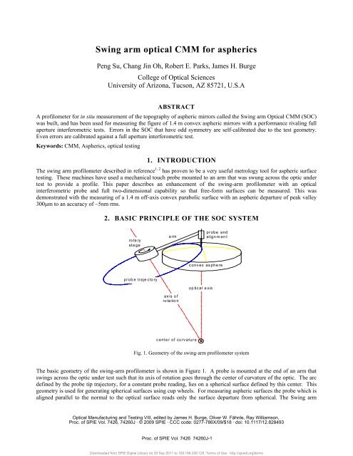
2. BASIC PRINCIPLE OF THE SOC SYSTEM
ro ta ry
sta ge
arm
probe and
alignm en t
convex asphere
probe trajectory
axis of
ro ta tio n
op tical axis
center of curvature
Fig. 1. Geometry of the swing-arm profilometer system
The basic geometry of the swing-arm profilometer is shown in Figure 1. A probe is mounted at the end of an arm that
swings across the optic under test such that its axis of rotation goes through the center of curvature of the optic. The arc
defined by the probe tip trajectory, for a constant probe reading, lies on a spherical surface defined by this center. This
geometry is used for generating spherical surfaces using cup wheels. For measuring aspheric surfaces the probe which is
aligned parallel to the normal to the optical surface reads only the surface departure from spherical. The Swing arm
Optical Manufacturing and Testing VIII, edited by James H. Burge, Oliver W. Fähnle, Ray Williamson,
Proc. of SPIE Vol. 7426, 74260J · © 2009 SPIE · CCC code: 0277-786X/09/$18 · doi: 10.1117/12.828493
Proc. of SPIE Vol. 7426 74260J-1
Downloaded from SPIE Digital Library on 29 Sep 2011 to 128.196.206.125. Terms of Use: http://spiedl.org/terms

Optical CMM (SOC) uses this simple geometry with an optical, non-contact interferometric probe that measures
continuously across the optic. The swing arm geometry works for convex, concave and plane parts. For measuring
concave parts, the scan angle need only be tilted towards the optic, rather than away from the optic as shown for the
convex measurements. In our shop, the SOC is rigidly mounted to a computer controlled polishing machine to allow in
situ measurements while the mirror is on the polishing table as shown in Fig. 2.
Fig. 2. SOC in situ measuring a 1.4-m convex off-axis parabolic mirror. Polishing head in back.
Fig. 3. SOC profiling pattern used for measuring the 1.4m convex asphere, coordinates units are mm
Fig. 3 shows the profiling pattern we used for measuring the 1.4m off-axis parabola (OAP). To be able to well sample
the high frequency structure in the mirror, the SOC makes 64 scans across the mirror, one arc every 5.625º in azimuth.
Since the arcs cross each other at eleven radial positions as the sensor scans the mirror edge to edge, we know the surface
Proc. of SPIE Vol. 7426 74260J-2
Downloaded from SPIE Digital Library on 29 Sep 2011 to 128.196.206.125. Terms of Use: http://spiedl.org/terms

heights must be the same at these scan crossings. This crossing height information is used to stitch the scans into a
surface with Maximum likelihood reconstruction method 3, 4 .
3. ALIGNMENT AND CALIBRATION OF THE SOC
The SOC system needs to be aligned so that the rotation axis passes through the nominal center curvature of the optic
under test to minimize the measurement dynamic range. Also, the probe position relative to the test optic needs to be
well known to be able to accurately reconstruct the topography of the test surface.
3.1 Alignment of the SOC
A coordinate system is set up using a laser tracker 5 with the OAP center as the origin and a surface normal at the center
as the z-axis. The x-axis joins the parent vertex to the OAP center. There are three laser tracker balls mounted to the
probe mount. By rotating the arm and reading out the tracker ball positions, the arm length and rotation axis angle can be
calculated in the OAP coordinate system. The 2-axis stage (elevation and azimuthal) that supports the SOC air bearing is
adjusted so that the rotation axis of the SOC passes through the center curvature of the mirror to null tilt and power from
the SOC scan. By iteratively scanning the surface and making adjustments, the SOC is aligned to minimize the probe
readout to find a best-fit sphere to the OAP. There is no intrinsic error from the alignment because the data reduction
process fully removes this 4 . The probe is aligned normal to the surface at the center of the OAP so that the probe will
measure the aspheric departure normal to the surface.
3.2 Determine probe coordinates
A laser tracker and a PSM 6 are used to calibrate the probe tip coordinates relative to the three tracker balls mounted
around it. After that a calibration between the tip coordinate and the swing arm bearing encoder readout is performed.
During a test only the encoder data and table angle are needed to find the probe tip in mirror coordinate system. After
getting the probe tip coordinate from encoder data, the measurement positions on the mirror during the scan can be
calculated with a simple ray tracing algorithm based on the mirror parameters.
3.3 Calibration of repeatable errors in the SOC 4
Errors with odd symmetry: 0.023 µm rms
Errors with even symmetry: 0.025 µm rms
Calibrated
measurement
error in µm
Normalized position on mirror
Normalized position on mirror
Fig. 4. (left) SOC errors with odd symmetry, with 0.023 µm rms magnitude. (right) errors with even symmetry, showing
0.025 µm rms.
As with any function, measurement errors in a single scan from SOC system can be divided into odd and even parts.
From the scan pattern shown in Fig. 3 we know that if all the scan data at different angles are averaged together, the odd
part due to the mirror will be zero, so the odd part of the average of the scans are entirely due to the odd errors in the
SOC. In this way, odd errors can be calibrated and removed during the data reduction.
Calibration data collected at different time, while the mirror was kept being polished, showed that the errors in SOC
system had a repeatability ~1nm rms. Fig 4 (left) shows an estimate of the odd error in our SOC system (low order linear
Proc. of SPIE Vol. 7426 74260J-3
Downloaded from SPIE Digital Library on 29 Sep 2011 to 128.196.206.125. Terms of Use: http://spiedl.org/terms

and cubic terms are removed). Currently, the even errors of SOC system are removed by calibration against an
independent full aperture interferometric test. Fig.4 (right) shows the even errors in our SOC system (quadratic error
removed).
4. SOC DATA REDUCTION AND TEST RESULT FOR AN OAP
An off-axis 1.4m convex parabola with 300 um aspheric departures was fabricated using the SOC system as the main
method of metrology. During a test the OAP was scanned in 64 equally spaced arcs. Each arc was scanned 8 times. The
data were then stitched together using a maximum likelihood reconstruction algorithm 3 that removes alignment errors.
Fig 5(a) shows an example of the raw data from a single scan. Fig 5 (b) shows the data with alignment errors removed.
Eight data sets are collected counting forward and backward scans at a single mirror angle during the test. Fig 5 (c)
shows the difference of a single forward scan data set from the average of that set of forward scan data; 6 nm rms is the
value. Considering a total of eight scans are used for calculating a single mirror angle data set, the data for stitching at
different mirror angles has a noise level of ~2nm rms.
150
data with alignment errors
5
individal scans
100
4
50
3
probe data (um)
0
-50
-100
-150
-200
um
2
1
0
-1
-250
-50 -40 -30 -20 -10 0 10 20
encoder data (degrees)
-2
-50 -40 -30 -20 -10 0 10 20
encoder angle
(a)
(b)
0.02
rms=6nm
0.015
0.01
Surface
measurement
in µm
0.005
0
-0.005
-0.01
-0.015
-0.02
-50 -40 -30 -20 -10 0 10 20
Encoder angle in degrees
Fig. 5. (a) Single scan of raw data, (b) scan data with alignment term removed, (c) departure of single scan from mean of
data set
(c)
Proc. of SPIE Vol. 7426 74260J-4
Downloaded from SPIE Digital Library on 29 Sep 2011 to 128.196.206.125. Terms of Use: http://spiedl.org/terms

4.1 Surface maps derived from the scan data
The data reduction program produces a surface map which is the departure from the ideal shape of the mirror. Fig 6
shows a comparison of the OAP test results from the SOC and the interferometric null test with astigmatism, coma and
trefoil removed from both tests (there are uncertainties of these three kinds of aberrations in the interferometric test due
to the test alignment). A direct subtraction of the maps shows a difference of ~ 9nm.
Fizeau=0.0357
SOC=0.0356
20
40
0.2
0.15
20
40
0.1
60
0.1
60
0.05
80
100
120
140
0.05
0
-0.05
80
100
120
140
0
-0.05
160
-0.1
160
-0.1
180
180
200
50 100 150 200
-0.15
200
50 100 150 200
(a)
(b)
20
40
60
80
100
120
140
160
180
200
differecne=0.0094
50 100 150 200
(c)
0.1
0.05
0
-0.05
-0.1
Fig. 6 Comparison of the interferometric Fizeau test data (a) and SOC data (b) with tilt, power, coma, astigmatism and
trefoil removed. The direct subtraction (c) shows only 9 nm rms
Proc. of SPIE Vol. 7426 74260J-5
Downloaded from SPIE Digital Library on 29 Sep 2011 to 128.196.206.125. Terms of Use: http://spiedl.org/terms

Fig. 7 shows a comparison of the high frequency information in the same data with the 43 lowest orders Zernike terms
removed. The difference is ~8nm.
Fizeau=0.0118
SOC=0.008
0.2
20
40
0.15
20
40
0.04
60
0.1
60
0.02
80
0.05
80
100
120
140
0
-0.05
100
120
140
0
-0.02
160
-0.1
160
-0.04
180
200
50 100 150 200
-0.15
180
200
50 100 150 200
-0.06
(a)
(b)
0.00786445
20
0.2
40
60
80
0.15
0.1
100
0.05
120
0
140
-0.05
160
180
200
50 100 150 200
-0.1
-0.15
(c)
Fig.7. Comparison of the interferometric Fizeau test data (a), SOC data (b) and difference (c) with 43 low order Zernike
aberration terms removed.
Proc. of SPIE Vol. 7426 74260J-6
Downloaded from SPIE Digital Library on 29 Sep 2011 to 128.196.206.125. Terms of Use: http://spiedl.org/terms

Fig. 8 shows a second set of data when the mirror closed to be finished. 43 low order Zernike terms are removed for the
comparison of the high frequency information in the data. The difference is ~5nm rms, better than the difference data
shown above since more careful interferometric data was taken to beat down the measurement noise. This difference
map is dominated by ghost fringes and known errors in the fold flat in the Fizeau test.
Fizeau 0.0085 um
SOC rms= 0.0062um
20
0.06
20
0.06
40
60
0.04
40
60
0.04
80
0.02
80
0.02
100
120
0
100
120
0
140
-0.02
140
-0.02
160
180
-0.04
160
180
-0.04
200
50 100 150 200
(a)
200
Differnce rms=0.0052um
50 100 150 200
(b)
20
40
60
80
100
120
140
160
180
0.08
0.06
0.04
0.02
0
-0.02
-0.04
200
50 100 150 200
-0.06
(c)
Fig. 8. Comparison of the final interferometric Fizeau test (a), the final SOC data (b) and the difference (c) with the 43 low
order Zernike terms removed.
Proc. of SPIE Vol. 7426 74260J-7
Downloaded from SPIE Digital Library on 29 Sep 2011 to 128.196.206.125. Terms of Use: http://spiedl.org/terms

Given a noise floor for the SOC data of ~2 nm rms as estimated from single scan data and comparisons with the Fizeau
data, an accuracy of better than 5 nm rms is a reasonable estimate for the performance of the SOC system.
5. SUMMARY
A profilometer (SOC) for in situ measurement of the topography of aspheric mirrors was developed at University of
Arizona, and has been used for measuring the figure of 1.4 m mirrors with a performance rivaling full aperture
interferometric tests. The SOC adopts swing-arm geometry that is a spherical coordinate system, is especially good at
testing optical elements since most of the interests are the departures from spheres. Only the radial scan motion needs to
be well controlled that is a simplification comparing with Cartesian coordinate system CMM. Further development
would add increased internal metrology, allowing complete self-calibration can be obtained for SOC. 4
REFERENCES
[1]
[2]
[3]
[4]
[5]
[6]
David S. Anderson, Robert E. Parks, and T. Shao, “A versatile profilometer for the measurement of aspherics,”
OF&T Workshop Technical Digest, Monterrey, CA (1990).
David S. Anderson and James H. Burge, Swing-arm profilometry of aspherics, Proc. SPIE. 2536, 169-179 (1995).
Peng Su, James H. Burge, Robert A. Sprowl, Jose Sasian, “Maximum likelihood estimation as a general method of
combining sub-aperture data for interferometric test,” Proc. SPIE. 6342, 63421x-1-63421x-6 (2006).
Peng Su, Chang Jin Oh, Robert E. Parks, James H. Burge, “Swing arm optical CMM,” to be submitted to Applied
Optics (2009).
James H. Burge, Peng Su, Chunyu Zhao, Tom Zobrist, “Use of a commercial laser tracker for optical alignment,”
Proc. SPIE. 6676, 66760E (2007).
Robert E. Parks, Versatile Auto-stigmatic Microscope. Proc. SPIE. 6290, 62890J (2006).
Proc. of SPIE Vol. 7426 74260J-8
Downloaded from SPIE Digital Library on 29 Sep 2011 to 128.196.206.125. Terms of Use: http://spiedl.org/terms