The Money Changing Problem Revisited - Universität Bielefeld
The Money Changing Problem Revisited - Universität Bielefeld
The Money Changing Problem Revisited - Universität Bielefeld

You also want an ePaper? Increase the reach of your titles
YUMPU automatically turns print PDFs into web optimized ePapers that Google loves.
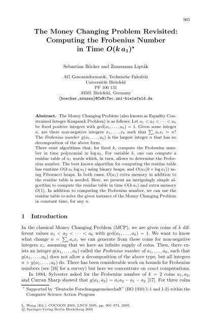
965<br />
<strong>The</strong> <strong>Money</strong> <strong>Changing</strong> <strong>Problem</strong> <strong>Revisited</strong>:<br />
Computing the Frobenius Number<br />
in Time O(ka 1 ) ⋆<br />
Sebastian Böcker and Zsuzsanna Lipták<br />
AG Genominformatik, Technische Fakultät<br />
Universität <strong>Bielefeld</strong><br />
PF 100 131<br />
33501 <strong>Bielefeld</strong>, Germany<br />
{boecker,zsuzsa}@CeBiTec.uni-bielefeld.de<br />
Abstract. <strong>The</strong> <strong>Money</strong> <strong>Changing</strong> <strong>Problem</strong> (also known as Equality Constrained<br />
Integer Knapsack <strong>Problem</strong>) is as follows: Let a 1
966 Sebastian Böcker and Zsuzsanna Lipták<br />
a 1 ,a 2 ,a 3 , Greenberg [9] provides a fast algorithm with runtime O(log a 1 ), and<br />
Davison [6] independently discovered a simple algorithm with runtime O(log a 2 ).<br />
Kannan [11] establishes algorithms that for any fixed k, compute the Frobenius<br />
number in time polynomial in log a k . For variable k, the runtime of such algorithms<br />
has a double exponential dependency on k, and is not competitive for<br />
k ≥ 5. Also, it does not appear that Kannan’s algorithms have actually been implemented.<br />
Computing the Frobenius number is NP-hard [15], so we cannot hope<br />
to find algorithms polynomial in k and log a k simultaneously unless P = NP.<br />
<strong>The</strong>re has been a considerable amount of research on computing the exact<br />
Frobenius number if k is variable, see again [16] for a survey. Heap and Lynn [10]<br />
suggest an algorithm with runtime O(a 3 k<br />
log g), and Wilf’s “circle-of-light” algorithm<br />
[18] runs in O(kg) time, where g = O(a 1 a k ) is the Frobenius number of the<br />
problem. Until recently, the fastest algorithm to compute g(a 1 ,...,a k ) was due<br />
to Nijenhuis [14]: It is based on Dijkstra’s method for computing shortest paths<br />
[7] using a priority queue. This algorithm has runtime O(ka 1 log a 1 ) using binary<br />
heaps, and O(a 1 (k+loga 1 )) using Fibonacci heaps as the priority queue. To find<br />
the Frobenius number, the algorithm computes a data structure (called “residue<br />
table” in the following) of a 1 words, which in turn allows simple computation of<br />
g(a 1 ,...,a k ). Nijenhuis’ algorithm requires O(a 1 ) extra memory in addition to<br />
the residue table. Recently, Beihoffer et al. [3] developed algorithms that work<br />
faster in practice, but none obtains asymptotically better runtime bounds than<br />
Nijenhuis’s algorithm, and all require extra memory linear in a 1 .<br />
Here, we present an intriguingly simple algorithm to compute the residue<br />
table – and hence, to find g(a 1 ,...,a k )–intimeO(ka 1 ) with constant extra<br />
memory. In addition to the improved runtime bound, our algorithm also outperforms<br />
Nijenhuis’ algorithm in practice.<br />
Moreover, access to the residue table allows us to solve subsequent MCP<br />
decision problems on the same coin set in constant time: Here, the input is<br />
a 1 ,...,a k ,n and we ask the question “Is n decomposable?” <strong>The</strong> MCP decision<br />
problem, also known as Equality Constrained Integer Knapsack <strong>Problem</strong>, is also<br />
NP-hard [13]. In principle, one can solve MCP decision problems using generating<br />
functions, but the computational cost for coefficient expansion and evaluation<br />
are too high in applications [8, Chapter 7.3]. It is computer science folklore<br />
that the question can be answered in time O(kn) using dynamic programming 1 ,<br />
but the linear runtime dependence on n is unfavorable. Aardal et al. [1, 2] use<br />
lattice basis reduction to find a decomposition of n. In Section 6 we show that<br />
computing the complete residue table using our algorithm is often faster than<br />
solving a single MCP decision instance with the method suggested by Aardal<br />
et al.<br />
We show in [4] that a slightly modified version of the algorithm presented<br />
here allows its application for the analysis of mass spectrometry data: <strong>The</strong>re, one<br />
is given a weighted alphabet (such as amino acids) and an input mass m, and<br />
one wants to find all decompositions of m. To this end, an “extended residue<br />
1 Wright [19] shows how to find a decomposition using a minimal number of coins in<br />
time O(kn)
<strong>The</strong> <strong>Money</strong> <strong>Changing</strong> <strong>Problem</strong> <strong>Revisited</strong> 967<br />
table” of size O(ka 1 ) is generated in runtime O(ka 1 ), where a 1 is the smallest<br />
mass in the alphabet and k the size of the alphabet. This data structure allows<br />
for computation of all decompositions in time linear in the size of the output,<br />
and otherwise independent of the input mass m. Confer [4] for details.<br />
2 Residue Classes and the Frobenius Number<br />
For integers a and b, let“a mod b” denote the unique integer p ∈{0,...,b− 1}<br />
such that p ≡ a (mod b) holds.<br />
Let a 1 < ···
968 Sebastian Böcker and Zsuzsanna Lipták<br />
p a 1 =5 a 2 =8 a 3 =9 a 4 =12<br />
0 0 0 0 0<br />
1 ∞ 16 16 16<br />
2 ∞ 32 17 12<br />
3 ∞ 8 8 8<br />
4 ∞ 24 9 9<br />
Fig. 1. Table n p for the MCP instance 5, 8, 9, 12<br />
In case all a 2 ,...,a k are coprime to a 1 , this short algorithm is already sufficient<br />
to find the correct values n p . We have displayed a small example in Figure 1,<br />
where every column corresponds to one iteration of the algorithm as described in<br />
the previous paragraph. For example, focus on the column a 3 = 9. We start with<br />
n = 0. In the first step, we have n ← 9andp =4.Sincenn 3 =8<br />
we set n ← 8. Third, we have n ← 8 + 9 = 17 and p =2.Sincenn 1 =16wesetn ← 16. Finally, we return to p =0vian ← 16 + 9 = 25.<br />
From the last column we can see that the Frobenius number for this example<br />
is g(5, 8, 9, 12) = 16 − 5 = 11.<br />
It is straighforward how to generalize the algorithm for d := gcd(a 1 ,a i ) > 1:<br />
In this case, we do the updating independently for every residue r =0,...,d−1:<br />
Only those n p for p ∈{0,...,a 1 − 1} are updated that satisfy p ≡ r (mod d).<br />
To guarantee that the round robin loop completes updating after a 1 /d steps, we<br />
have to start the loop from a minimal n p with p ≡ r (mod d). For r =0we<br />
know that n 0 = 0 is the unique minimum, while for r ≠0wesearchforthe<br />
minimum first.<br />
Round Robin Algorithm<br />
1 initialize n 0 =0andn p = ∞ for p =1,...,a 1 − 1<br />
2 for i =2,...,k do<br />
3 d =gcd(a 1 ,a i );<br />
4 for r =0,...,d− 1do<br />
5 Find n =min{n q | q mod d = r, 0 ≤ q ≤ a 1 − 1}<br />
6 If n 1.<br />
Lemma 1. Suppose that n ′ p for p =0,...,a 1−1 are the correct residue table entries<br />
for the MCP instance a 1 ,...,a k−1 .Initializen p ← n ′ p for p =0,...,a 1 −1.
<strong>The</strong> <strong>Money</strong> <strong>Changing</strong> <strong>Problem</strong> <strong>Revisited</strong> 969<br />
<strong>The</strong>n, after one iteration of the outer loop (lines 3–10) of the Round Robin Algorithm,<br />
the residue table entries equal the values n p for p =0,...,a 1 − 1 for<br />
the MCP instance a 1 ,...,a k .<br />
Since for k =1,n 0 =0andn p = ∞ for p ≠ 0 are the correct values for<br />
the MCP with one coin, we can use induction to show the correctness of the<br />
algorithm. To prove the lemma, we first note that for all p =0,...,a 1 − 1,<br />
n p ≤ n ′ p and n p ≤ n q + a k for q =(p − a k )moda 1<br />
after termination. Assume that for some n, there exists a decomposition n =<br />
∑ k<br />
i=1 a ix i .Wehavetoshown ≥ n p for p = n mod a 1 .Now, ∑ k−1<br />
i=1 a ix i =<br />
n − a k x k is a decomposition of the MCP instance a 1 ,...,a k−1 and for q =<br />
(n − a k x k )moda 1 we have n − a k x k ≥ n ′ q. We conclude<br />
n p ≤ n q + a k x k ≤ n ′ q + a kx k ≤ n.<br />
By an analogous argument, we infer n p = n for minimal such n. One can easily<br />
show that n p = ∞ if and only if no n with n ≡ p (mod a 1 ) has a decomposition<br />
with respect to the MCP instance a 1 ,...,a k .<br />
Under the standard model of computation, time and space complexity of the<br />
algorithm are immediate and we reach:<br />
<strong>The</strong>orem 1. <strong>The</strong> Round Robin Algorithm computes the residue table of an instance<br />
a 1 ,...,a k of the <strong>Money</strong> <strong>Changing</strong> <strong>Problem</strong>, in runtime Θ(ka 1 ) and extra<br />
memory O(1).<br />
To obtain a decomposition of any n in k steps, we save for every p =<br />
0,...,a 1 − 1 the minimal index i such that a decomposition x 1 ,...,x k of n p<br />
has x i > 0, and we also save the maximal x i for any such decomposition. This<br />
can be easily incorporated into the algorithm retaining identical time complexity,<br />
and requires 2a 1 additional words of memory. Doing so, we obtain a lexicographically<br />
maximal decomposition. Note that unlike the Change Making <strong>Problem</strong>,<br />
we do not try to minimize the number of coins used.<br />
4 Heuristic Runtime Improvements<br />
We can improve the Round Robin Algorithm in the following ways: First, we do<br />
not have to explicitly compute the greatest common divisor gcd(a 1 ,a i ). Instead,<br />
we do the first round robin loop (lines 6–9) for r =0withn = n 0 = p =0until<br />
we reach n = p = 0 again. We count the number of steps t to this point. <strong>The</strong>n,<br />
d =gcd(a 1 ,a i )= a1<br />
t<br />
and for d>1, we do the remaining round robin loops<br />
r =1,...,d− 1.<br />
Second, for r>0 we do not have to explicitly search for the minimum in<br />
N r := {n q : q = r, r + d, r +2d,...,r+(a 1 − d)}. Instead, we start with n = n r<br />
and do exactly t − 1 steps of the round robin loop. Here, n r = ∞ may hold, so
970 Sebastian Böcker and Zsuzsanna Lipták<br />
we initialize p = r (line 5) and update p ← (p + a i )moda 1 separately in line 7.<br />
Afterwards, we continue with this loop until we first encounter some n p ≤ n in<br />
line 8, and stop there. <strong>The</strong> second loop takes at most t−1 steps, because at some<br />
stage we reach the minimal n p =minN r and then, n p
<strong>The</strong> <strong>Money</strong> <strong>Changing</strong> <strong>Problem</strong> <strong>Revisited</strong> 971<br />
instance of the problem if run in cache memory. For an instance a 1 ,...,a k of<br />
MCP, the runtime t mod of our modified algorithm roughly depends on the values<br />
1/ gcd(a 1 ,a i ):<br />
t mod ≈ t cache +(t mem − t cache )<br />
1<br />
k − 1<br />
k∑<br />
i=2<br />
1<br />
gcd(a 1 ,a i ) .<br />
For random integers u, v uniformly drawn from {1,...,n} we estimate (analogously<br />
to [12], Section 4.5.2)<br />
( )<br />
1<br />
n∑ p 1<br />
n<br />
E<br />
≈<br />
gcd(u, v) d 2 d = p ∑ 1<br />
d 3 = pH(3) n with p =6/π 2 ,<br />
d=1<br />
d=1<br />
where the H n (3) are the harmonic numbers of third order. <strong>The</strong> H n<br />
(3) form a monotonically<br />
increasing series with 1.2020
972 Sebastian Böcker and Zsuzsanna Lipták<br />
6 Computational Results<br />
We generated 12 000 random instances of MCP, with k =5, 10, 20 and 10 3 ≤<br />
a i ≤ 10 7 . We have plotted the runtime of the optimized Round Robin Algorithm<br />
against a 1 in Figure 3. As expected, the runtime of the algorithm is mostly<br />
independent of the structure of the underlying instance. <strong>The</strong> processor cache, on<br />
the contrary, is responsible for major runtime differences. <strong>The</strong> left plot contains<br />
only those instances with a 1 ≤ 10 6 ; here, the residue table of size a 1 appears<br />
to fit into the processor cache. <strong>The</strong> right plot contains all random instances; for<br />
a 1 > 10 6 , the residue table has to be stored in main memory.<br />
6<br />
RoundRobin<br />
200<br />
RoundRobin<br />
5<br />
Nijenhuis<br />
k=20<br />
Nijenhuis<br />
k=20<br />
4<br />
k=10<br />
150<br />
time [sec]<br />
k=5<br />
3<br />
time [sec]<br />
k=10<br />
100<br />
2<br />
k=5<br />
50<br />
k=20<br />
1<br />
k=20<br />
k=10<br />
k=10<br />
k=5<br />
k=5<br />
0<br />
0 2*10 5 4*10 5 6*10 5 8*10 5 1*10 6 0<br />
0 2*10 6 4*10 6 6*10 6 8*10 6 1*10 7<br />
Fig. 3. Runtime vs. a 1 for k =5, 10, 20 where a 1 ≤ 10 6 (left) and a 1 ≤ 10 7 (right)<br />
To compare runtimes of the Round Robin Algorithm with those of Nijenhuis’<br />
algorithm [14], we re-implemented the latter in C++ using a binary heap as<br />
the priority queue. As one can see in Figure 3, the speedup of our optimized<br />
algorithm is about 10-fold for a 1 ≤ 10 6 , and more than threefold otherwise.<br />
Regarding Kannan’s algorithm [11], the runtime factor k kk > 10 2184 for k =5<br />
makes it impossible to use this approach.<br />
Comparing the original Round Robin Algorithm with the optimized version,<br />
the achieved speedup was 1.67-fold on average (data not shown).<br />
We also tested our algorithm on some instances of the <strong>Money</strong> <strong>Changing</strong><br />
<strong>Problem</strong> that are known to be “hard”: Twenty-five examples with 5 ≤ k ≤ 10<br />
and 3719 ≤ a 1 ≤ 48709 were taken from [2], along with runtimes given there<br />
for standard linear programming based branch-and-bound search. <strong>The</strong> runtime<br />
of the optimized Round Robin Algorithm (900 MHz UltraSparc III processor,<br />
C++) for every instance is below 10 ms, see Table 1. Note that in [2], Aardal and<br />
Lenstra do not compute the Frobenius number g but only verify that g cannot<br />
be decomposed. In contrast, the Round Robin Algorithm computes the residue<br />
table of the instance, which in turn allows to answer all subsequent questions<br />
whether some n is decomposable, in constant time. Still and all, runtimes usually<br />
compare well to those of [2] and clearly outperform LP-based branch-and-bound<br />
search (all runtimes above 9000 ms), taking into account the threefold processor<br />
power running the Round Robin Algorithm.
<strong>The</strong> <strong>Money</strong> <strong>Changing</strong> <strong>Problem</strong> <strong>Revisited</strong> 973<br />
Table 1. Runtimes on instances from [2] in milliseconds, measured on a 359 MHz<br />
UltraSparc II (Aardal & Lenstra) and on a 900 MHz UltraSparc III (Round Robin)<br />
Instance c1 c2 c3 c4 c5 p1 p2 p3 p4 p5 p6 p7 p8<br />
Aardal & Lenstra 1 1 1 1 1 1 1 2 1 2 1 2 1<br />
Round Robin 0.8 0.9 0.9 1.1 1.6 3.1 1.2 4.9 9.2 4.0 3.4 3.1 2.8<br />
Instance p9 p10 p11 p12 p13 p14 p15 p16 p17 p18 p19 p20<br />
Aardal & Lenstra 3 2 5 12 6 12 80 80 150 120 100 5<br />
Round Robin 0.4 6.5 1.8 2.1 2.4 1.8 2.1 6.4 2.5 3.7 3.2 9.0<br />
7 Conclusion<br />
We have presented the Round Robin Algorithm that generates a residue table<br />
which allows us to find the Frobenius number, as well as to answer whether any<br />
number n can be decomposed, the latter in constant time. <strong>The</strong> advantages of<br />
our algorithm are (i) its simplicity, making it easy to implement and allowing<br />
further improvements; (ii) its guaranteed worst case runtime of O(ka 1 ), independent<br />
of the structure of the underlying instance; and (iii) its constant extra<br />
memory requirements. To the best of our knowledge, no other algorithm with<br />
worst case runtime O(ka 1 ) is known. In addition, runtimes of the Round Robin<br />
Algorithm compare well to other, more sophisticated approaches, see [3]. It is<br />
rather surprising that despite the simplicity and efficiency of the Round Robin<br />
algorithm, it has not been reported in literature.<br />
Simulations clearly show that the time consuming part of the Round Robin<br />
algorithm is accessing memory. We are currently working on a modification that<br />
performs cache-optimized memory access as described in Section 5, even when<br />
gcd(a 1 ,a i ) is small.<br />
As mentioned in the introduction, we can use a slightly modified version of<br />
the Round Robin Algorithm to compute a data structure, which in turns allows<br />
us to find all decompositions of any input n. To this end, we generate an extended<br />
residue table of size O(ka 1 )inruntimeO(ka 1 ) that stores not only the<br />
“final” column of the residue table, but also all intermediate steps, confer Fig. 1.<br />
If we denote the number of decompositions of n by γ(n), then this data structure<br />
allows us to generate all decompositions in time O(ka 1 γ(n)) backtracking<br />
through the extended residue table, see [4].<br />
Acknowledgments<br />
Implementation and simulations by Henner Sudek. We thank Stan Wagon and<br />
Albert Nijenhuis for helpful discussions.<br />
References<br />
1. K. Aardal, C. Hurkens, and A. K. Lenstra. Solving a system of diophantine equations<br />
with lower and upper bounds on the variables. Math. Operations Research,<br />
25:427–442, 2000.
974 Sebastian Böcker and Zsuzsanna Lipták<br />
2. K. Aardal and A. K. Lenstra. Hard equality constrained integer knapsacks. Lect.<br />
Notes Comput. Sc., 2337:350–366, 2002.<br />
3. D. E. Beihoffer, J. Hendry, A. Nijenhuis, and S. Wagon. Faster algorithms for<br />
Frobenius numbers. In preparation.<br />
4. S. Böcker and Zs. Lipták. Efficient mass decomposition. In Proc. of ACM Symposium<br />
on Applied Computing 2005, pages 151–157, Santa Fe, USA, 2005.<br />
5. A. Brauer and J. E. Shockley. On a problem of Frobenius. J. Reine Angew. Math.,<br />
211:215–220, 1962.<br />
6. J. L. Davison. On the linear diophantine problem of Frobenius. J. Number <strong>The</strong>ory,<br />
48(3):353–363, 1994.<br />
7. E. Dijkstra. A note on two problems in connexion with graphs. Numerische<br />
Mathematik, 1:269–271, 1959.<br />
8. R. L. Graham, D. E. Knuth, and O. Patashnik. Concrete Mathematics. Addison-<br />
Wesley, Reading, Massachusetts, second edition, 1994.<br />
9. H. Greenberg. Solution to a linear diophantine equation for nonnegative integers.<br />
J. Algorithms, 9(3):343–353, 1988.<br />
10. B. R. Heap and M. S. Lynn. A graph-theoretic algorithm for the solution of a<br />
linear diophantine problem of Frobenius. Numer. Math., 6:346–354, 1964.<br />
11. R. Kannan. Lattice translates of a polytope and the Frobenius problem. Combinatorica,<br />
12:161–177, 1991.<br />
12. D. E. Knuth. <strong>The</strong> Art of Computer Programming: Seminumerical Algorithms,<br />
volume 2. Addison-Wesley, Reading, Massachusetts, third edition, 1997.<br />
13. G. S. Lueker. Two NP-complete problems in nonnegative integer programming.<br />
Technical Report TR-178, Department of Electrical Engineering, Princeton University,<br />
March 1975.<br />
14. A. Nijenhuis. A minimal-path algorithm for the “money changing problem”. Amer.<br />
Math. Monthly, 86:832–835, 1979. Correction in Amer. Math. Monthly, 87:377,<br />
1980.<br />
15. J. L. Ramírez-Alfonsín. Complexity of the Frobenius problem. Combinatorica,<br />
16(1):143–147, 1996.<br />
16. J. L. Ramírez-Alfonsín. <strong>The</strong> Diophantine Frobenius <strong>Problem</strong>. Oxford University<br />
Press, 2005. To appear.<br />
17. J. J. Sylvester and W. J. Curran Sharp. <strong>Problem</strong> 7382. Educational Times, 37:26,<br />
1884.<br />
18. H. S. Wilf. A circle-of-lights algorithm for the “money-changing problem”. Amer.<br />
Math. Monthly, 85:562–565, 1978.<br />
19. J. W. Wright. <strong>The</strong> change-making problem. J. Assoc. Comput. Mach., 22(1):125–<br />
128, 1975.