Pattern Recognition and Machine Learning

Pattern Recognition and Machine Learning
Solutions to the Exercises: Web-Edition
Markus Svensén and Christopher M. Bishop
c○ Markus Svensén and Christopher M. Bishop (2002–2007).
All rights retained. Not to be redistributed without permission
March 23, 2007

Pattern Recognition and Machine Learning
Solutions to the Exercises: Web-Edition
Markus Svensén and Christopher M. Bishop
Copyright c○ 2002–2007
This is an early partial release of the solutions manual (web-edition) for the book Pattern Recognition and
Machine Learning (PRML; published by Springer in 2006). It contains solutions to the www exercises
in PRML for chapters 1–4. This release was created March 23, 2007; further releases with solutions to
later chapters will be published in due course on the PRML web-site (see below).
The authors would like to express their gratitude to the various people who have provided feedback on
pre-releases of this document. In particular, the “Bishop Reading Group”, held in the Visual Geometry
Group at the University of Oxford provided valuable comments and suggestions.
Please send any comments, questions or suggestions about the solutions in this document to Markus
Svensén, markussv@microsoft.com.
Further information about PRML is available from:
http://research.microsoft.com/∼cmbishop/PRML

Contents
Contents 5
Chapter 1: Pattern Recognition . . . . . . . . . . . . . . . . . . . . . . . 7
Chapter 2: Density Estimation . . . . . . . . . . . . . . . . . . . . . . . 19
Chapter 3: Linear Models for Regression . . . . . . . . . . . . . . . . . . 34
Chapter 4: Linear Models for Classification . . . . . . . . . . . . . . . . 41
5

6 CONTENTS

Solutions 1.1– 1.4 7
Chapter 1 Pattern Recognition
1.1 Substituting (1.1) into (1.2) and then differentiating with respect to w i we obtain
(
N∑ ∑ M
w j x j n − t n
)x i n = 0. (1)
n=1
j=0
Re-arranging terms then gives the required result.
1.4 We are often interested in finding the most probable value for some quantity. In
the case of probability distributions over discrete variables this poses little problem.
However, for continuous variables there is a subtlety arising from the nature of probability
densities and the way they transform under non-linear changes of variable.
Consider first the way a function f(x) behaves when we change to a new variable y
where the two variables are related by x = g(y). This defines a new function of y
given by
˜f(y) = f(g(y)). (2)
Suppose f(x) has a mode (i.e. a maximum) at ̂x so that f ′ (̂x) = 0. The corresponding
mode of ˜f(y) will occur for a value ŷ obtained by differentiating both sides of
(2) with respect to y
˜f ′ (ŷ) = f ′ (g(ŷ))g ′ (ŷ) = 0. (3)
Assuming g ′ (ŷ) ≠ 0 at the mode, then f ′ (g(ŷ)) = 0. However, we know that
f ′ (̂x) = 0, and so we see that the locations of the mode expressed in terms of each
of the variables x and y are related by ̂x = g(ŷ), as one would expect. Thus, finding
a mode with respect to the variable x is completely equivalent to first transforming
to the variable y, then finding a mode with respect to y, and then transforming back
to x.
Now consider the behaviour of a probability density p x (x) under the change of variables
x = g(y), where the density with respect to the new variable is p y (y) and is
given by ((1.27)). Let us write g ′ (y) = s|g ′ (y)| where s ∈ {−1, +1}. Then ((1.27))
can be written
p y (y) = p x (g(y))sg ′ (y).
Differentiating both sides with respect to y then gives
p ′ y(y) = sp ′ x(g(y)){g ′ (y)} 2 + sp x (g(y))g ′′ (y). (4)
Due to the presence of the second term on the right hand side of (4) the relationship
̂x = g(ŷ) no longer holds. Thus the value of x obtained by maximizing p x (x) will
not be the value obtained by transforming to p y (y) then maximizing with respect to
y and then transforming back to x. This causes modes of densities to be dependent
on the choice of variables. In the case of linear transformation, the second term

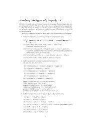
8 Solution 1.7
Figure 1
Example of the transformation of
the mode of a density under a nonlinear
change of variables, illustrating
the different behaviour compared
to a simple function. See the
text for details.
y
1
p y (y)
g −1 (x)
0.5
p x (x)
0
0 5 x 10
vanishes on the right hand side of (4) vanishes, and so the location of the maximum
transforms according to ̂x = g(ŷ).
This effect can be illustrated with a simple example, as shown in Figure 1. We
begin by considering a Gaussian distribution p x (x) over x with mean µ = 6 and
standard deviation σ = 1, shown by the red curve in Figure 1. Next we draw a
sample of N = 50, 000 points from this distribution and plot a histogram of their
values, which as expected agrees with the distribution p x (x).
Now consider a non-linear change of variables from x to y given by
The inverse of this function is given by
x = g(y) = ln(y) − ln(1 − y) + 5. (5)
y = g −1 (x) =
1
1 + exp(−x + 5)
(6)
which is a logistic sigmoid function, and is shown in Figure 1 by the blue curve.
If we simply transform p x (x) as a function of x we obtain the green curve p x (g(y))
shown in Figure 1, and we see that the mode of the density p x (x) is transformed
via the sigmoid function to the mode of this curve. However, the density over y
transforms instead according to (1.27) and is shown by the magenta curve on the left
side of the diagram. Note that this has its mode shifted relative to the mode of the
green curve.
To confirm this result we take our sample of 50, 000 values of x, evaluate the corresponding
values of y using (6), and then plot a histogram of their values. We see that
this histogram matches the magenta curve in Figure 1 and not the green curve!
1.7 The transformation from Cartesian to polar coordinates is defined by
x = r cosθ (7)
y = r sin θ (8)

Solution 1.8 9
and hence we have x 2 + y 2 = r 2 where we have used the well-known trigonometric
result (2.177). Also the Jacobian of the change of variables is easily seen to be
∂x ∂x
∂(x, y)
∂r ∂θ
=
∂(r, θ)
∂y ∂y
∣ ∣
∂r ∂θ
=
cosθ −r sin θ
∣ sin θ r cosθ ∣ = r
where again we have used (2.177). Thus the double integral in (1.125) becomes
∫ 2π ∫ ∞
( )
I 2 = exp − r2
r dr dθ (9)
0 0
2σ 2
∫ ∞ (
= 2π exp − u ) 1
du (10)
0
2σ 2 2
[ (
= π exp − u ) (−2σ )] ∞
2
(11)
2σ 2 0
= 2πσ 2 (12)
where we have used the change of variables r 2 = u. Thus
I = ( 2πσ 2) 1/2
.
Finally, using the transformation y = x −µ, the integral of the Gaussian distribution
becomes
∫ ∞
N ( x|µ, σ 2) ∫
1 ∞
( )
dx =
exp − y2
dy
−∞
(2πσ 2 ) 1/2 −∞ 2σ 2
I
=
(2πσ 2 ) = 1 1/2
as required.
1.8 From the definition (1.46) of the univariate Gaussian distribution, we have
∫ ∞
( ) 1/2 { 1
E[x] =
exp − 1 }
2πσ 2 2σ 2(x − µ)2 x dx. (13)
−∞
Now change variables using y = x − µ to give
∫ ∞
( ) 1/2 { 1
E[x] =
exp − 1 }
(y + µ) dy. (14)
2πσ 2 2σ 2y2
−∞
We now note that in the factor (y + µ) the first term in y corresponds to an odd
integrand and so this integral must vanish (to show this explicitly, write the integral

10 Solutions 1.9– 1.10
as the sum of two integrals, one from −∞ to 0 and the other from 0 to ∞ and then
show that these two integrals cancel). In the second term, µ is a constant and pulls
outside the integral, leaving a normalized Gaussian distribution which integrates to
1, and so we obtain (1.49).
To derive (1.50) we first substitute the expression (1.46) for the normal distribution
into the normalization result (1.48) and re-arrange to obtain
∫ ∞
exp
−∞
{
− 1
2σ 2(x − µ)2 }
dx = ( 2πσ 2) 1/2
. (15)
We now differentiate both sides of (15) with respect to σ 2 and then re-arrange to
obtain
( ) 1/2 ∫ 1
∞
{
exp − 1 }
2πσ 2 2σ 2(x − µ)2 (x − µ) 2 dx = σ 2 (16)
which directly shows that
−∞
Now we expand the square on the left-hand side giving
E[(x − µ) 2 ] = var[x] = σ 2 . (17)
E[x 2 ] − 2µE[x] + µ 2 = σ 2 .
Making use of (1.49) then gives (1.50) as required.
Finally, (1.51) follows directly from (1.49) and (1.50)
E[x 2 ] − E[x] 2 = ( µ 2 + σ 2) − µ 2 = σ 2 .
1.9 For the univariate case, we simply differentiate (1.46) with respect to x to obtain
d
dx N ( x|µ, σ 2) = −N ( x|µ, σ 2) x − µ
.
σ 2
Setting this to zero we obtain x = µ.
Similarly, for the multivariate case we differentiate (1.52) with respect to x to obtain
∂
∂x N(x|µ,Σ) = −1 2 N(x|µ,Σ)∇ {
x (x − µ) T Σ −1 (x − µ) }
= −N(x|µ,Σ)Σ −1 (x − µ),
where we have used (C.19), (C.20) and the fact that Σ −1 is symmetric. Setting this
derivative equal to 0, and left-multiplying by Σ, leads to the solution x = µ.
1.10 Since x and z are independent, their joint distribution factorizes p(x, z) = p(x)p(z),
and so
∫∫
E[x + z] = (x + z)p(x)p(z) dxdz (18)
∫ ∫
= xp(x) dx + zp(z) dz (19)
= E[x] + E[z]. (20)

Solutions 1.12– 1.15 11
Similarly for the variances, we first note that
(x + z − E[x + z]) 2 = (x − E[x]) 2 + (z − E[z]) 2 + 2(x − E[x])(z − E[z]) (21)
where the final term will integrate to zero with respect to the factorized distribution
p(x)p(z). Hence
∫∫
var[x + z] = (x + z − E[x + z]) 2 p(x)p(z) dxdz
∫
∫
= (x − E[x]) 2 p(x) dx + (z − E[z]) 2 p(z) dz
= var(x) + var(z). (22)
For discrete variables the integrals are replaced by summations, and the same results
are again obtained.
1.12 If m = n then x n x m = x 2 n and using (1.50) we obtain E[x 2 n] = µ 2 + σ 2 , whereas if
n ≠ m then the two data points x n and x m are independent and hence E[x n x m ] =
E[x n ]E[x m ] = µ 2 where we have used (1.49). Combining these two results we
obtain (1.130).
Next we have
using (1.49).
E[µ ML ] = 1 N
N∑
E[x n ] = µ (23)
n=1
Finally, consider E[σML 2 ]. From (1.55) and (1.56), and making use of (1.130), we
have
⎡ ( ) 2
⎤
E[σML] 2 = E⎣ 1 N∑
x n − 1 N∑
x m
⎦
N N
n=1 m=1
[
= 1 N∑
E x 2 n
N
− 2 N∑
N x n x m + 1
N
]
∑ N∑
x
N 2 m x l
n=1
m=1 m=1 l=1
{ (µ 2 + 1 )
N σ2 + µ 2 + 1 }
N σ2
as required.
=
=
µ 2 + σ 2 − 2
( ) N − 1
σ 2 (24)
N
1.15 The redundancy in the coefficients in (1.133) arises from interchange symmetries
between the indices i k . Such symmetries can therefore be removed by enforcing an
ordering on the indices, as in (1.134), so that only one member in each group of
equivalent configurations occurs in the summation.

12 Solution 1.15
To derive (1.135) we note that the number of independent parameters n(D, M)
which appear at order M can be written as
n(D, M) =
D∑
i 1
∑
i 1 =1 i 2 =1
i 1 =1
i 2 =1
· · ·
i∑
M−1
i M =1
which has M terms. This can clearly also be written as
{
D∑ i1 i
∑ M−1
}
∑
n(D, M) = · · · 1
i M =1
1 (25)
where the term in braces has M−1 terms and which, from (25), must equal n(i 1 , M−
1). Thus we can write
which is equivalent to (1.135).
n(D, M) =
(26)
D∑
n(i 1 , M − 1) (27)
i 1 =1
To prove (1.136) we first set D = 1 on both sides of the equation, and make use of
0! = 1, which gives the value 1 on both sides, thus showing the equation is valid for
D = 1. Now we assume that it is true for a specific value of dimensionality D and
then show that it must be true for dimensionality D + 1. Thus consider the left-hand
side of (1.136) evaluated for D + 1 which gives
D+1
∑
i=1
(i + M − 2)!
(i − 1)!(M − 1)!
=
=
=
(D + M − 1)!
(D − 1)!M!
+
(D + M − 1)!
D!(M − 1)!
(D + M − 1)!D + (D + M − 1)!M
D!M!
(D + M)!
D!M!
which equals the right hand side of (1.136) for dimensionality D + 1. Thus, by
induction, (1.136) must hold true for all values of D.
Finally we use induction to prove (1.137). For M = 2 we find obtain the standard
result n(D, 2) = 1 D(D + 1), which is also proved in Exercise 1.14. Now assume
2
that (1.137) is correct for a specific order M − 1 so that
n(D, M − 1) =
Substituting this into the right hand side of (1.135) we obtain
(28)
(D + M − 2)!
(D − 1)! (M − 1)! . (29)
n(D, M) =
D∑
i=1
(i + M − 2)!
(i − 1)! (M − 1)!
(30)

Solutions 1.17– 1.20 13
which, making use of (1.136), gives
n(D, M) =
(D + M − 1)!
(D − 1)! M!
and hence shows that (1.137) is true for polynomials of order M. Thus by induction
(1.137) must be true for all values of M.
1.17 Using integration by parts we have
Γ(x + 1) =
For x = 1 we have
∫ ∞
0
u x e −u du
(31)
= [ −e −u u x] ∫ ∞
∞
+ xu x−1 e −u du = 0 + xΓ(x). (32)
0
Γ(1) =
∫ ∞
0
0
e −u du = [ −e −u] ∞
0
= 1. (33)
If x is an integer we can apply proof by induction to relate the gamma function to
the factorial function. Suppose that Γ(x + 1) = x! holds. Then from the result (32)
we have Γ(x + 2) = (x + 1)Γ(x + 1) = (x + 1)!. Finally, Γ(1) = 1 = 0!, which
completes the proof by induction.
1.18 On the right-hand side of (1.142) we make the change of variables u = r 2 to give
1
2 S D
∫ ∞
0
e −u u D/2−1 du = 1 2 S DΓ(D/2) (34)
where we have used the definition (1.141) of the Gamma function. On the left hand
side of (1.142) we can use (1.126) to obtain π D/2 . Equating these we obtain the
desired result (1.143).
The volume of a sphere of radius 1 in D-dimensions is obtained by integration
V D = S D
∫ 1
For D = 2 and D = 3 we obtain the following results
0
r D−1 dr = S D
D . (35)
S 2 = 2π, S 3 = 4π, V 2 = πa 2 , V 3 = 4 3 πa3 . (36)
1.20 Since p(x) is radially symmetric it will be roughly constant over the shell of radius
r and thickness ɛ. This shell has volume S D r D−1 ɛ and since ‖x‖ 2 = r 2 we have
∫
p(x) dx ≃ p(r)S D r D−1 ɛ (37)
shell

14 Solutions 1.22– 1.24
from which we obtain (1.148). We can find the stationary points of p(r) by differentiation
d
[
(
dr p(r) ∝ (D − 1)r D−2 + r D−1 − r ( )
)]exp − r2
= 0. (38)
σ 2 2σ 2
Solving for r, and using D ≫ 1, we obtain ̂r ≃ √ Dσ.
Next we note that
]
p(̂r + ɛ) ∝ (̂r + ɛ) D−1 (̂r + ɛ)2
exp
[−
2σ
[
2 ]
(̂r + ɛ)2
= exp − + (D − 1) ln(̂r + ɛ) . (39)
2σ 2
We now expand p(r) around the point ̂r. Since this is a stationary point of p(r)
we must keep terms up to second order. Making use of the expansion ln(1 + x) =
x − x 2 /2 + O(x 3 ), together with D ≫ 1, we obtain (1.149).
Finally, from (1.147) we see that the probability density at the origin is given by
p(x = 0) =
1
(2πσ 2 ) 1/2
while the density at ‖x‖ = ̂r is given from (1.147) by
( )
1
p(‖x‖ = ̂r) =
(2πσ 2 ) exp − ̂r2 1
=
(− 1/2 2σ 2 (2πσ 2 ) exp D )
1/2 2
where we have used ̂r ≃ √ Dσ. Thus the ratio of densities is given by exp(D/2).
1.22 Substituting L kj = 1 − δ kj into (1.81), and using the fact that the posterior probabilities
sum to one, we find that, for each x we should choose the class j for which
1 − p(C j |x) is a minimum, which is equivalent to choosing the j for which the posterior
probability p(C j |x) is a maximum. This loss matrix assigns a loss of one if
the example is misclassified, and a loss of zero if it is correctly classified, and hence
minimizing the expected loss will minimize the misclassification rate.
1.24 A vector x belongs to class C k with probability p(C k |x). If we decide to assign x to
class C j we will incur an expected loss of ∑ k L kjp(C k |x), whereas if we select the
reject option we will incur a loss of λ. Thus, if
j = arg min
l
∑
L kl p(C k |x) (40)
then we minimize the expected loss if we take the following action
{ ∑
class j, if minl
choose
k L klp(C k |x) < λ;
reject, otherwise.
k
(41)

Solutions 1.25– 1.27 15
CHECK! 1.25
For a loss matrix L kj = 1 − I kj we have ∑ k L klp(C k |x) = 1 − p(C l |x) and so we
reject unless the smallest value of 1 − p(C l |x) is less than λ, or equivalently if the
largest value of p(C l |x) is less than 1 − λ. In the standard reject criterion we reject
if the largest posterior probability is less than θ. Thus these two criteria for rejection
are equivalent provided θ = 1 − λ.
The expected squared loss for a vectorial target variable is given by
∫∫
E[L] = ‖y(x) − t‖ 2 p(t,x) dxdt.
Our goal is to choose y(x) so as to minimize E[L]. We can do this formally using
the calculus of variations to give
∫
δE[L]
δy(x) = 2(y(x) − t)p(t,x) dt = 0.
Solving for y(x), and using the sum and product rules of probability, we obtain
∫
tp(t,x) dt ∫
y(x) = ∫ = tp(t|x) dt
p(t,x) dt
which is the conditional average of t conditioned on x. For the case of a scalar target
variable we have
∫
y(x) = tp(t|x) dt
which is equivalent to (1.89).
1.27 Since we can choose y(x) independently for each value of x, the minimum of the
expected L q loss can be found by minimizing the integrand given by
∫
|y(x) − t| q p(t|x) dt (42)
for each value of x. Setting the derivative of (42) with respect to y(x) to zero gives
the stationarity condition
∫
q|y(x) − t| q−1 sign(y(x) − t)p(t|x) dt
= q
∫ y(x)
−∞
∫ ∞
|y(x) − t| q−1 p(t|x) dt − q |y(x) − t| q−1 p(t|x) dt = 0
y(x)
which can also be obtained directly by setting the functional derivative of (1.91) with
respect to y(x) equal to zero. It follows that y(x) must satisfy
∫ y(x)
−∞
|y(x) − t| q−1 p(t|x) dt =
∫ ∞
|y(x) − t| q−1 p(t|x) dt. (43)
y(x)

16 Solutions 1.29– 1.31
For the case of q = 1 this reduces to
∫ y(x)
−∞
p(t|x) dt =
∫ ∞
which says that y(x) must is the conditional median of t.
p(t|x) dt. (44)
y(x)
For q → 0 we note that, as a function of t, the quantity |y(x) − t| q is close to 1
everywhere except in a small neighbourhood around t = y(x) where it falls to zero.
The value of (42) will therefore be close to 1, since the density p(t) is normalized, but
reduced slightly by the ‘notch’ close to t = y(x). We obtain the biggest reduction in
(42) by choosing the location of the notch to coincide with the largest value of p(t),
i.e. with the (conditional) mode.
1.29 The entropy of an M-state discrete variable x can be written in the form
M∑
M∑ 1
H(x) = − p(x i ) lnp(x i ) = p(x i ) ln
p(x i ) . (45)
i=1
The function ln(x) is concave⌢ and so we can apply Jensen’s inequality in the form
(1.115) but with the inequality reversed, so that
( M
)
∑ 1
H(x) ln p(x i ) = lnM. (46)
p(x i )
i=1
1.31 We first make use of the relation I(x;y) = H(y) − H(y|x) which we obtained in
(1.121), and note that the mutual information satisfies I(x;y) 0 since it is a form
of Kullback-Leibler divergence. Finally we make use of the relation (1.112) to obtain
the desired result (1.152).
To show that statistical independence is a sufficient condition for the equality to be
satisfied, we substitute p(x,y) = p(x)p(y) into the definition of the entropy, giving
∫∫
H(x,y) = p(x,y) lnp(x,y) dxdy
∫∫
= p(x)p(y) {ln p(x) + lnp(y)} dxdy
∫
∫
= p(x) lnp(x) dx + p(y) lnp(y) dy
= H(x) + H(y).
To show that statistical independence is a necessary condition, we combine the equality
condition
H(x,y) = H(x) + H(y)
with the result (1.112) to give
i=1
H(y|x) = H(y).

Solution 1.34 17
We now note that the right-hand side is independent of x and hence the left-hand side
must also be constant with respect to x. Using (1.121) it then follows that the mutual
information I[x,y] = 0. Finally, using (1.120) we see that the mutual information is
a form of KL divergence, and this vanishes only if the two distributions are equal, so
that p(x,y) = p(x)p(y) as required.
1.34 Obtaining the required functional derivative can be done simply by inspection. However,
if a more formal approach is required we can proceed as follows using the
techniques set out in Appendix D. Consider first the functional
∫
I[p(x)] = p(x)f(x) dx.
Under a small variation p(x) → p(x) + ɛη(x) we have
∫
∫
I[p(x) + ɛη(x)] = p(x)f(x) dx + ɛ
η(x)f(x) dx
and hence from (D.3) we deduce that the functional derivative is given by
Similarly, if we define
∫
J[p(x)] =
δI
δp(x) = f(x).
p(x) lnp(x) dx
then under a small variation p(x) → p(x) + ɛη(x) we have
∫
J[p(x) + ɛη(x)] = p(x) lnp(x) dx
{∫
∫
}
1
+ɛ η(x) lnp(x) dx + p(x)
p(x) η(x) dx + O(ɛ 2 )
and hence
δJ
= p(x) + 1.
δp(x)
Using these two results we obtain the following result for the functional derivative
Re-arranging then gives (1.108).
− lnp(x) − 1 + λ 1 + λ 2 x + λ 3 (x − µ) 2 .
To eliminate the Lagrange multipliers we substitute (1.108) into each of the three
constraints (1.105), (1.106) and (1.107) in turn. The solution is most easily obtained
by comparison with the standard form of the Gaussian, and noting that the results
λ 1 = 1 − 1 2 ln( 2πσ 2) (47)
λ 2 = 0 (48)
1
λ 3 =
(49)
2σ 2

18 Solutions 1.35– 1.38
do indeed satisfy the three constraints.
Note that there is a typographical error in the question, which should read ”Use
calculus of variations to show that the stationary point of the functional shown just
before (1.108) is given by (1.108)”.
For the multivariate version of this derivation, see Exercise 2.14.
1.35 Substituting the right hand side of (1.109) in the argument of the logarithm on the
right hand side of (1.103), we obtain
∫
H[x] = − p(x) lnp(x) dx
∫
= − p(x)
(− 1 )
(x − µ)2
2 ln(2πσ2 ) − dx
2σ 2
= 1 (ln(2πσ 2 ) + 1 ∫
)
p(x)(x − µ) 2 dx
2 σ 2
= 1 2
(
ln(2πσ 2 ) + 1 ) ,
where in the last step we used (1.107).
1.38 From (1.114) we know that the result (1.115) holds for M = 1. We now suppose that
it holds for some general value M and show that it must therefore hold for M + 1.
Consider the left hand side of (1.115)
( M+1
) (
)
∑ M∑
f λ i x i = f λ M+1 x M+1 + λ i x i (50)
i=1
i=1
(
)
M∑
= f λ M+1 x M+1 + (1 − λ M+1 ) η i x i (51)
where we have defined
η i =
i=1
λ i
1 − λ M+1
. (52)
We now apply (1.114) to give
( M+1
) ( ∑ M
)
∑
f λ i x i λ M+1 f(x M+1 ) + (1 − λ M+1 )f η i x i . (53)
i=1
i=1
We now note that the quantities λ i by definition satisfy
M+1
∑
i=1
λ i = 1 (54)

Solutions 1.41– 2.1 19
and hence we have
M∑
λ i = 1 − λ M+1 (55)
i=1
Then using (52) we see that the quantities η i satisfy the property
M∑
η i =
i=1
1 ∑ M
λ i = 1. (56)
1 − λ M+1
i=1
Thus we can apply the result (1.115) at order M and so (53) becomes
f
( M+1
) ∑
λ i x i λ M+1 f(x M+1 )+(1−λ M+1 )
i=1
where we have made use of (52).
M∑
η i f(x i ) =
i=1
M+1
∑
i=1
λ i f(x i ) (57)
1.41 From the product rule we have p(x,y) = p(y|x)p(x), and so (1.120) can be written
as
∫∫
∫∫
I(x;y) = − p(x,y) lnp(y) dxdy + p(x,y) lnp(y|x) dx dy
∫
∫∫
= − p(y) lnp(y) dy + p(x,y) lnp(y|x) dxdy
= H(y) − H(y|x). (58)
Chapter 2 Density Estimation
2.1 From the definition (2.2) of the Bernoulli distribution we have
∑
p(x|µ) = p(x = 0|µ) + p(x = 1|µ) (59)
∑
x∈{0,1}
x∈{0,1}
= (1 − µ) + µ = 1 (60)
∑
xp(x|µ) = 0.p(x = 0|µ) + 1.p(x = 1|µ) = µ (61)
x∈{0,1}
(x − µ) 2 p(x|µ) = µ 2 p(x = 0|µ) + (1 − µ) 2 p(x = 1|µ) (62)
= µ 2 (1 − µ) + (1 − µ) 2 µ = µ(1 − µ). (63)

20 Solution 2.3
The entropy is given by
H(x) = −
∑
x∈{0,1}
= − ∑
x∈{0,1}
p(x|µ) lnp(x|µ)
µ x (1 − µ) 1−x {x lnµ + (1 − x) ln(1 − µ)}
= −(1 − µ) ln(1 − µ) − µ lnµ. (64)
2.3 Using the definition (2.10) we have
( ( )
N N N!
+ =
n)
n − 1 n!(N − n)! + N!
(n − 1)!(N + 1 − n)!
(N + 1 − n)N! + nN! (N + 1)!
= =
n!(N + 1 − n)! n!(N + 1 − n)!
( ) N + 1
= . (65)
n
To prove the binomial theorem (2.263) we note that the theorem is trivially true
for N = 0. We now assume that it holds for some general value N and prove its
correctness for N + 1, which can be done as follows
N∑
( N
(1 + x) N+1 = (1 + x) x
n)
n
=
=
=
=
n=0
N∑
( N
x
n)
n +
n=0
( N
0
)
x 0 +
N+1
∑
n=1
N∑
{( N
+
n)
n=1
( ) N
x n
n − 1
( N
n − 1
)
)}
x n +
( N
N)
x N+1
( ) N + 1
N∑
( ( )
N + 1 N + 1
x 0 + x n + x N+1
0
n N + 1
n=1
N+1
∑
( ) N + 1
x n (66)
n
n=0
which completes the inductive proof. Finally, using the binomial theorem, the normalization
condition (2.264) for the binomial distribution gives
N∑
( N ∑ N ( )( ) n
N µ
µ
n)
n (1 − µ) N−n = (1 − µ) N n 1 − µ
n=0
n=0
(
= (1 − µ) N 1 + µ ) N
= 1 (67)
1 − µ

Solutions 2.5– 2.9 21
Figure 2 Plot of the region of integration of (68)
in (x,t) space.
t
t = x
x
as required.
2.5 Making the change of variable t = y + x in (2.266) we obtain
∫ ∞
{∫ ∞
}
Γ(a)Γ(b) = x a−1 exp(−t)(t − x) b−1 dt dx. (68)
0
x
We now exchange the order of integration, taking care over the limits of integration
Γ(a)Γ(b) =
∫ ∞ ∫ t
0
0
x a−1 exp(−t)(t − x) b−1 dx dt. (69)
The change in the limits of integration in going from (68) to (69) can be understood
by reference to Figure 2. Finally we change variables in the x integral using x = tµ
to give
Γ(a)Γ(b) =
∫ ∞
0
= Γ(a + b)
exp(−t)t a−1 t b−1 t dt
∫ 1
0
∫ 1
0
µ a−1 (1 − µ) b−1 dµ
µ a−1 (1 − µ) b−1 dµ. (70)
2.9 When we integrate over µ M−1 the lower limit of integration is 0, while the upper
limit is 1 − ∑ M−2
j=1 µ j since the remaining probabilities must sum to one (see Figure
2.4). Thus we have
p M−1 (µ 1 , . . .,µ M−2 ) =
[ M−2 ∏
= C M µ α k−1
k
k=1
∫ 1−
0
M−2
j=1 µ j
] ∫ 1−
M−2
j=1 µ j
0
p M (µ 1 , . . .,µ M−1 ) dµ M−1
µ α M−1−1
M−1
(
1 −
M−1
∑
j=1
µ j
) αM −1
dµ M−1 .

22 Solution 2.11
In order to make the limits of integration equal to 0 and 1 we change integration
variable from µ M−1 to t using
( )
M−2
∑
µ M−1 = t 1 − µ j (71)
which gives
p M−1 (µ 1 , . . .,µ M−2 )
[ M−2 ∏
= C M µ α k−1
k
k=1
](
1 −
[ M−2
]( ∏
= C M µ α k−1
k
1 −
k=1
M−2
∑
j=1
M−2
∑
j=1
j=1
) αM−1 +α M −1 ∫ 1
µ j t αM−1−1 (1 − t) α M −1 dt
µ j
) αM−1 +α M −1
Γ(αM−1 )Γ(α M )
Γ(α M−1 + α M )
where we have used (2.265). The right hand side of (72) is seen to be a normalized
Dirichlet distribution over M −1 variables, with coefficients α 1 , . . .,α M−2 , α M−1 +
α M , (note that we have effectively combined the final two categories) and we can
identify its normalization coefficient using (2.38). Thus
as required.
Γ(α 1 + . . . + α M )
C M =
Γ(α 1 ) . . .Γ(α M−2 )Γ(α M−1 + α M ) · Γ(α M−1 + α M )
Γ(α M−1 )Γ(α M )
= Γ(α 1 + . . . + α M )
Γ(α 1 ) . . .Γ(α M )
2.11 We first of all write the Dirichlet distribution (2.38) in the form
where
Dir(µ|α) = K(α)
K(α) =
Next we note the following relation
∂ ∏ M
∂α j
k=1
µ α k−1
k
=
=
M∏
k=1
µ α k−1
k
Γ(α 0 )
Γ(α 1 ) · · ·Γ(α M ) .
∂ ∏ M
exp ((α k − 1) lnµ k )
∂α j
k=1
M∏
lnµ j exp {(α k − 1) lnµ k }
k=1
= lnµ j
M
∏
k=1
µ α k−1
k
0
(72)
(73)

Solution 2.14 23
from which we obtain
E[ln µ j ] = K(α)
∫ 1
0
· · ·
∫ 1
= K(α) ∂ ∫ 1
· · ·
∂α j
= K(α) ∂
∂µ k
1
K(α)
= − ∂
∂µ k
lnK(α).
0
0
lnµ j
M
∏
∫ 1
0
k=1
M∏
k=1
µ α k−1
k
dµ 1 . . . dµ M
µ α k−1
k
dµ 1 . . . dµ M
Finally, using the expression for K(α), together with the definition of the digamma
function ψ(·), we have
E[ln µ j ] = ψ(α k ) − ψ(α 0 ).
2.14 As for the univariate Gaussian considered in Section 1.6, we can make use of Lagrange
multipliers to enforce the constraints on the maximum entropy solution. Note
that we need a single Lagrange multiplier for the normalization constraint (2.280),
a D-dimensional vector m of Lagrange multipliers for the D constraints given by
(2.281), and a D ×D matrix L of Lagrange multipliers to enforce the D 2 constraints
represented by (2.282). Thus we maximize
∫
(∫ )
˜H[p] = − p(x) lnp(x) dx + λ p(x) dx − 1
(∫ )
+m T p(x)x dx − µ
{ (∫
)}
+Tr L p(x)(x − µ)(x − µ) T dx − Σ . (74)
By functional differentiation (Appendix D) the maximum of this functional with
respect to p(x) occurs when
0 = −1 − lnp(x) + λ + m T x + Tr{L(x − µ)(x − µ) T }. (75)
Solving for p(x) we obtain
p(x) = exp { λ − 1 + m T x + (x − µ) T L(x − µ) } . (76)
We now find the values of the Lagrange multipliers by applying the constraints. First
we complete the square inside the exponential, which becomes
λ − 1 +
(
x − µ + 1 2 L−1 m) T
L
(
x − µ + 1 2 L−1 m
)
+ µ T m − 1 4 mT L −1 m.

24 Solution 2.16
We now make the change of variable
y = x − µ + 1 2 L−1 m.
The constraint (2.281) then becomes
∫ {
exp λ − 1 + y T Ly + µ T m − 1 }(
4 mT L −1 m y + µ − 1 )
2 L−1 m dy = µ.
In the final parentheses, the term in y vanishes by symmetry, while the term in µ
simply integrates to µ by virtue of the normalization constraint (2.280) which now
takes the form
∫ {
exp λ − 1 + y T Ly + µ T m − 1 }
4 mT L −1 m dy = 1.
and hence we have
− 1 2 L−1 m = 0
where again we have made use of the constraint (2.280). Thus m = 0 and so the
density becomes
p(x) = exp { λ − 1 + (x − µ) T L(x − µ) } .
Substituting this into the final constraint (2.282), and making the change of variable
x − µ = z we obtain
∫
exp { λ − 1 + z T Lz } zz T dx = Σ.
Applying an analogous argument to that used to derive (2.64) we obtain L = − 1 Σ. 2
Finally, the value of λ is simply that value needed to ensure that the Gaussian distribution
is correctly normalized, as derived in Section 2.3, and hence is given by
{ } 1 1
λ − 1 = ln
.
(2π) D/2 |Σ| 1/2
2.16 We have p(x 1 ) = N(x 1 |µ 1 , τ −1
1 ) and p(x 2 ) = N(x 2 |µ 2 , τ −1
2 ). Since x = x 1 + x 2
we also have p(x|x 2 ) = N(x|µ 1 + x 2 , τ −1
1 ). We now evaluate the convolution
integral given by (2.284) which takes the form
p(x) =
( τ1
2π
) 1/2 ( τ2
2π
) 1/2
∫ ∞
exp
−∞
{
− τ 1
2 (x − µ 1 − x 2 ) 2 − τ 2
2 (x 2 − µ 2 ) 2 }
dx 2 .
(77)
Since the final result will be a Gaussian distribution for p(x) we need only evaluate
its precision, since, from (1.110), the entropy is determined by the variance or equivalently
the precision, and is independent of the mean. This allows us to simplify the
calculation by ignoring such things as normalization constants.

Solutions 2.17– 2.20 25
We begin by considering the terms in the exponent of (77) which depend on x 2 which
are given by
− 1 2 x2 2 (τ 1 + τ 2 ) + x 2 {τ 1 (x − µ 1 ) + τ 2 µ 2 }
= − 1 {
2 (τ 1 + τ 2 ) x 2 − τ } 2
1(x − µ 1 ) + τ 2 µ 2
+ {τ 1(x − µ 1 ) + τ 2 µ 2 } 2
τ 1 + τ 2 2(τ 1 + τ 2 )
where we have completed the square over x 2 . When we integrate out x 2 , the first
term on the right hand side will simply give rise to a constant factor independent
of x. The second term, when expanded out, will involve a term in x 2 . Since the
precision of x is given directly in terms of the coefficient of x 2 in the exponent, it is
only such terms that we need to consider. There is one other term in x 2 arising from
the original exponent in (77). Combining these we have
− τ 1
2 x2 +
τ 2 1
2(τ 1 + τ 2 ) x2 = − 1 τ 1 τ 2
x 2
2 τ 1 + τ 2
from which we see that x has precision τ 1 τ 2 /(τ 1 + τ 2 ).
We can also obtain this result for the precision directly by appealing to the general
result (2.115) for the convolution of two linear-Gaussian distributions.
The entropy of x is then given, from (1.110), by
H(x) = 1 { }
2 ln 2π(τ1 + τ 2 )
. (78)
τ 1 τ 2
2.17 We can use an analogous argument to that used in the solution of Exercise 1.14.
Consider a general square matrix Λ with elements Λ ij . Then we can always write
Λ = Λ A + Λ S where
Λ S ij = Λ ij + Λ ji
, Λ A ij = Λ ij − Λ ji
2
2
and it is easily verified that Λ S is symmetric so that Λ S ij = ΛS ji , and ΛA is antisymmetric
so that Λ A ij = −ΛS ji . The quadratic form in the exponent of a D-dimensional
multivariate Gaussian distribution can be written
1
D∑ D∑
(x i − µ i )Λ ij (x j − µ j ) (80)
2
i=1 j=1
where Λ = Σ −1 is the precision matrix. When we substitute Λ = Λ A + Λ S into
(80) we see that the term involving Λ A vanishes since for every positive term there
is an equal and opposite negative term. Thus we can always take Λ to be symmetric.
2.20 Since u 1 , . . .,u D constitute a basis for R D , we can write
a = â 1 u 1 + â 2 u 2 + . . . + â D u D ,
(79)

26 Solutions 2.22– 2.24
where â 1 , . . .,â D are coefficients obtained by projecting a on u 1 , . . .,u D . Note that
they typically do not equal the elements of a.
Using this we can write
a T Σa = ( â 1 u T 1 + . . . + â Du T D) Σ (â1 u 1 + . . . + â D u D )
and combining this result with (2.45) we get
) (â1 u T 1 + . . . + â D u T D (â1 λ 1 u 1 + . . . + â D λ D u D ).
Now, since u T i u j = 1 only if i = j, and 0 otherwise, this becomes
â 2 1 λ 1 + . . . + â 2 D λ D
and since a is real, we see that this expression will be strictly positive for any nonzero
a, if all eigenvalues are strictly positive. It is also clear that if an eigenvalue,
λ i , is zero or negative, there exist a vector a (e.g. a = u i ), for which this expression
will be less than or equal to zero. Thus, that a matrix has eigenvectors which are all
strictly positive is a sufficient and necessary condition for the matrix to be positive
definite.
2.22 Consider a matrix M which is symmetric, so that M T = M. The inverse matrix
M −1 satisfies
MM −1 = I.
Taking the transpose of both sides of this equation, and using the relation (C.1), we
obtain
(
M
−1 ) T
M T = I T = I
since the identity matrix is symmetric. Making use of the symmetry condition for
M we then have ( M
−1 ) T
M = I
and hence, from the definition of the matrix inverse,
(
M
−1 ) T
= M
−1
and so M −1 is also a symmetric matrix.
2.24 Multiplying the left hand side of (2.76) by the matrix (2.287) trivially gives the identity
matrix. On the right hand side consider the four blocks of the resulting partitioned
matrix:
upper left
upper right
AM − BD −1 CM = (A − BD −1 C)(A − BD −1 C) −1 = I (81)
−AMBD −1 + BD −1 + BD −1 CMBD −1
= −(A − BD −1 C)(A − BD −1 C) −1 BD −1 + BD −1
= −BD −1 + BD −1 = 0 (82)

Solutions 2.28– 2.32 27
lower left
CM − DD −1 CM = CM − CM = 0 (83)
lower right
−CMBD −1 + DD −1 + DD −1 CMBD −1 = DD −1 = I. (84)
Thus the right hand side also equals the identity matrix.
2.28 For the marginal distribution p(x) we see from (2.92) that the mean is given by the
upper partition of (2.108) which is simply µ. Similarly from (2.93) we see that the
covariance is given by the top left partition of (2.105) and is therefore given by Λ −1 .
Now consider the conditional distribution p(y|x). Applying the result (2.81) for the
conditional mean we obtain
µ y|x = Aµ + b + AΛ −1 Λ(x − µ) = Ax + b.
Similarly applying the result (2.82) for the covariance of the conditional distribution
we have
as required.
cov[y|x] = L −1 + AΛ −1 A T − AΛ −1 ΛΛ −1 A T = L −1
2.32 The quadratic form in the exponential of the joint distribution is given by
− 1 2 (x − µ)T Λ(x − µ) − 1 2 (y − Ax − b)T L(y − Ax − b). (85)
We now extract all of those terms involving x and assemble them into a standard
Gaussian quadratic form by completing the square
where
= − 1 2 xT (Λ + A T LA)x + x T [ Λµ + A T L(y − b) ] + const
= − 1 2 (x − m)T (Λ + A T LA)(x − m)
+ 1 2 mT (Λ + A T LA)m + const (86)
m = (Λ + A T LA) −1 [ Λµ + A T L(y − b) ] .
We can now perform the integration over x which eliminates the first term in (86).
Then we extract the terms in y from the final term in (86) and combine these with
the remaining terms from the quadratic form (85) which depend on y to give
= − 1 2 yT { L − LA(Λ + A T LA) −1 A T L } y
+y T [{ L − LA(Λ + A T LA) −1 A T L } b
+LA(Λ + A T LA) −1 Λµ ] . (87)

28 Solution 2.34
We can identify the precision of the marginal distribution p(y) from the second order
term in y. To find the corresponding covariance, we take the inverse of the precision
and apply the Woodbury inversion formula (2.289) to give
{
L − LA(Λ + A T LA) −1 A T L } −1
= L −1 + AΛ −1 A T (88)
which corresponds to (2.110).
Next we identify the mean ν of the marginal distribution. To do this we make use of
(88) in (87) and then complete the square to give
where
− 1 2 (y − ν)T ( L −1 + AΛ −1 A T) −1
(y − ν) + const
ν = ( L −1 + AΛ −1 A T) [ (L −1 + AΛ −1 A T ) −1 b + LA(Λ + A T LA) −1 Λµ ] .
Now consider the two terms in the square brackets, the first one involving b and the
second involving µ. The first of these contribution simply gives b, while the term in
µ can be written
= ( L −1 + AΛ −1 A T) LA(Λ + A T LA) −1 Λµ
= A(I + Λ −1 A T LA)(I + Λ −1 A T LA) −1 Λ −1 Λµ = Aµ
where we have used the general result (BC) −1 = C −1 B −1 . Hence we obtain
(2.109).
2.34 Differentiating (2.118) with respect to Σ we obtain two terms:
− N 2
∂
∂Σ ln |Σ| − 1 ∂
2 ∂Σ
N∑
(x n − µ) T Σ −1 (x n − µ).
n=1
For the first term, we can apply (C.28) directly to get
− N 2
∂
∂Σ ln |Σ| = −N 2
For the second term, we first re-write the sum
(
Σ
−1 ) T
= −
N
2 Σ−1 .
N∑
(x n − µ) T Σ −1 (x n − µ) = NTr [ Σ −1 S ] ,
n=1
where
S = 1 N
N∑
(x n − µ)(x n − µ) T .
n=1

Solution 2.36 29
Using this together with (C.21), in which x = Σ ij (element (i, j) in Σ), and properties
of the trace we get
∂
∂Σ ij
N
∑
n=1
(x n − µ) T Σ −1 (x n − µ) = N ∂ Tr [ Σ −1 S ]
∂Σ ij
[ ] ∂
= NTr Σ −1 S
∂Σ ij
[ ]
= −NTr Σ −1 ∂Σ
Σ −1 S
∂Σ ij
[ ]
∂Σ
= −NTr Σ −1 SΣ −1
∂Σ ij
= −N ( Σ −1 SΣ −1) ij
where we have used (C.26). Note that in the last step we have ignored the fact that
Σ ij = Σ ji , so that ∂Σ/∂Σ ij has a 1 in position (i, j) only and 0 everywhere else.
Treating this result as valid nevertheless, we get
− 1 ∂
2 ∂Σ
N∑
(x n − µ) T Σ −1 (x n − µ) = N 2 Σ−1 SΣ −1 .
n=1
Combining the derivatives of the two terms and setting the result to zero, we obtain
Re-arrangement then yields
as required.
N
2 Σ−1 = N 2 Σ−1 SΣ −1 .
Σ = S
2.36 Consider the expression for σ(N) 2 and separate out the contribution from observation
x N to give
σ 2 (N) = 1 N
N∑
(x n − µ) 2
n=1
= 1 N−1
∑
(x n − µ) 2 + (x N − µ) 2
N
N
n=1
= N − 1
N σ2 (N−1) + (x N − µ) 2
N
= σ 2 (N−1) − 1 N σ2 (N−1) + (x N − µ) 2
N
= σ(N−1) 2 + 1 { }
(xN − µ) 2 − σ(N−1)
2 . (89)
N

30 Solution 2.40
If we substitute the expression for a Gaussian distribution into the result (2.135) for
the Robbins-Monro procedure applied to maximizing likelihood, we obtain
{
}
= σ(N−1) 2 + a ∂
N−1 − 1 2 ln σ2 (N−1) − (x N − µ) 2
σ 2 (N)
= σ 2 (N−1) + a N−1
∂σ 2 (N−1)
{
−
1
2σ 2 (N−1)
}
+ (x N − µ) 2
2σ 4 (N−1)
2σ 2 (N−1)
= σ(N−1) 2 + a N−1
{ }
(xN − µ) 2 − σ 2
2σ(N−1)
4 (N−1) . (90)
Comparison of (90) with (89) allows us to identify
a N−1 = 2σ4 (N−1)
N . (91)
Note that the sign in (2.129) is incorrect, and this equation should read
θ (N) = θ (N−1) − a N−1 z(θ (N−1) ).
Also, in order to be consistent with the assumption that f(θ) > 0 for θ > θ ⋆ and
f(θ) < 0 for θ < θ ⋆ in Figure 2.10, we should find the root of the expected negative
log likelihood in (2.133). Finally, the labels µ and µ ML in Figure 2.11 should be
interchanged.
2.40 The posterior distribution is proportional to the product of the prior and the likelihood
function
N∏
p(µ|X) ∝ p(µ) p(x n |µ,Σ). (92)
Thus the posterior is proportional to an exponential of a quadratic form in µ given
by
− 1 2 (µ − µ 0) T Σ −1
0 (µ − µ 0 ) − 1 2
n=1
N∑
(x n − µ) T Σ −1 (x n − µ)
n=1
= − 1 ( (
2 µT Σ −1
0 + NΣ −1) N
)
∑
µ + µ T Σ −1
0 µ 0 + Σ −1 x n + const
where ‘const.’ denotes terms independent of µ. Using the discussion following
(2.71) we see that the mean and covariance of the posterior distribution are given by
n=1
µ N = ( Σ −1
0 + NΣ −1) −1 ( )
Σ
−1
0 µ 0 + Σ −1 Nµ ML
Σ −1
N
(93)
= Σ −1
0 + NΣ −1 (94)

Solutions 2.46– 2.47 31
where µ ML is the maximum likelihood solution for the mean given by
µ ML = 1 N
N∑
x n . (95)
n=1
2.46 From (2.158), we have
∫ ∞
0
b a e (−bτ) τ a−1 ( τ
) 1/2
exp
{− τ }
Γ(a) 2π 2 (x − µ)2 dτ
( ) 1/2 ∫
= ba 1
∞
{ ( )}
τ a−1/2 (x − µ)2
exp −τ b + dτ.
Γ(a) 2π
2
0
We now make the proposed change of variable z = τ∆, where ∆ = b+(x −µ) 2 /2,
yielding
( )
b a 1/2 ∫ 1
∞
∆ −a−1/2
Γ(a) 2π
0
z a−1/2 exp(−z) dz
( ) 1/2
= ba 1
∆ −a−1/2 Γ(a + 1/2)
Γ(a) 2π
where we have used the definition of the Gamma function (1.141). Finally, we substitute
b + (x − µ) 2 /2 for ∆, ν/2 for a and ν/2λ for b:
Γ(−a + 1/2)
Γ(a)
=
=
=
Γ ((ν + 1)/2)
Γ(ν/2)
Γ ((ν + 1)/2)
Γ(ν/2)
Γ ((ν + 1)/2)
Γ(ν/2)
( ) 1/2
1
b a ∆ a−1/2
2π
( ν
) ν/2
( ) 1/2 ( 1 ν (x − µ)2
+
2λ 2π 2λ 2
( ν
) ν/2
( ) 1/2
1
( ν
) −(ν+1)/2
(1 +
2λ 2π 2λ
( ) 1/2 ( ) −(ν+1)/2
λ λ(x − µ)2
1 +
νπ
ν
) −(ν+1)/2
) −(ν+1)/2
λ(x − µ)2
ν
2.47 Ignoring the normalization constant, we write (2.159) as
[
λ(x − µ)2
St(x|µ, λ, ν) ∝ 1 +
ν
(
= exp − ν − 1 ln
[1 +
2
] −(ν−1)/2
])
λ(x − µ)2
. (96)
ν

32 Solutions 2.51– 2.56
For large ν, we make use of the Taylor expansion for the logarithm in the form
ln(1 + ɛ) = ɛ + O(ɛ 2 ) (97)
to re-write (96) as
(
exp − ν − 1 [ ])
λ(x − µ)2
ln 1 +
2 ν
(
= exp − ν − 1 [ ])
λ(x − µ)
2
+ O(ν −2 )
2 ν
(
)
λ(x − µ)2
= exp − + O(ν −1 ) .
2
We see that in the limit ν → ∞ this becomes, up to an overall constant, the same as
a Gaussian distribution with mean µ and precision λ. Since the Student distribution
is normalized to unity for all values of ν it follows that it must remain normalized in
this limit. The normalization coefficient is given by the standard expression (2.42)
for a univariate Gaussian.
2.51 Using the relation (2.296) we have
1 = exp(iA) exp(−iA) = (cosA + i sin A)(cos A − i sin A) = cos 2 A + sin 2 A.
Similarly, we have
Finally
cos(A − B) = R exp{i(A − B)}
= R exp(iA) exp(−iB)
= R(cosA + i sin A)(cosB − i sin B)
= cosAcosB + sin A sin B.
sin(A − B) = I exp{i(A − B)}
= I exp(iA) exp(−iB)
= I(cosA + i sin A)(cosB − i sin B)
= sin A cos B − cosAsin B.
2.56 We can most conveniently cast distributions into standard exponential family form by
taking the exponential of the logarithm of the distribution. For the Beta distribution
(2.13) we have
Beta(µ|a, b) =
Γ(a + b)
exp {(a − 1) lnµ + (b − 1) ln(1 − µ)} (98)
Γ(a)Γ(b)

Solution 2.60 33
which we can identify as being in standard exponential form (2.194) with
h(µ) = 1 (99)
Γ(a + b)
g(a, b) = (100)
Γ(a)Γ(b)
( )
lnµ
u(µ) =
(101)
ln(1 − µ)
( )
a − 1
η(a, b) = . (102)
b − 1
Applying the same approach to the gamma distribution (2.146) we obtain
from which it follows that
Gam(λ|a, b) = ba
exp {(a − 1) lnλ − bλ}.
Γ(a)
h(λ) = 1 (103)
g(a, b) =
u(λ) =
η(a, b) =
b a
(104)
Γ(a)
( )
λ
(105)
lnλ
( )
−b
. (106)
a − 1
Finally, for the von Mises distribution (2.179) we make use of the identity (2.178) to
give
1
p(θ|θ 0 , m) =
2πI 0 (m) exp {m cosθ cosθ 0 + m sin θ sin θ 0 }
from which we find
h(θ) = 1 (107)
1
g(θ 0 , m) =
(108)
2πI 0 (m)
( )
cosθ
u(θ) =
(109)
sin θ
( )
m cosθ0
η(θ 0 , m) = . (110)
m sinθ 0
2.60 The value of the density p(x) at a point x n is given by h j(n) , where the notation j(n)
denotes that data point x n falls within region j. Thus the log likelihood function
takes the form
N∑
N∑
lnp(x n ) = lnh j(n) .
n=1
n=1

34 Solution 3.1
We now need to take account of the constraint that p(x) must integrate to unity. Since
p(x) has the constant value h i over region i, which has volume ∆ i , the normalization
constraint becomes ∑ i h i∆ i = 1. Introducing a Lagrange multiplier λ we then
minimize the function
with respect to h k to give
(
N∑ ∑
lnh j(n) + λ
i
n=1
0 = n k
h k
+ λ∆ k
h i ∆ i − 1
where n k denotes the total number of data points falling within region k. Multiplying
both sides by h k , summing over k and making use of the normalization constraint,
we obtain λ = −N. Eliminating λ then gives our final result for the maximum
likelihood solution for h k in the form
h k = n k
N
1
∆ k
.
Note that, for equal sized bins ∆ k = ∆ we obtain a bin height h k which is proportional
to the fraction of points falling within that bin, as expected.
)
Chapter 3 Linear Models for Regression
3.1 Using (3.6), we have
2σ(2a) − 1 =
=
2
1 + e − 1 −2a
2 1 + e−2a
−
1 + e−2a 1 + e −2a
= 1 − e−2a
1 + e −2a
= ea − e −a
e a + e −a
= tanh(a)

Solution 3.4 35
3.4 Let
If we now take a j = (x − µ j )/2s, we can rewrite (3.101) as
y(x,w) = w 0 +
= w 0 +
= u 0 +
M∑
w j σ(2a j )
j=1
M∑
j=1
w j
2 (2σ(2a j) − 1 + 1)
M∑
u j tanh(a j ),
j=1
where u j = w j /2, for j = 1, . . .,M, and u 0 = w 0 + ∑ M
j=1 w j/2. Note that there is
a typographical error in the question: there is a 2 missing in the denominator of the
argument to the ‘tanh’ function in equation (3.102).
ỹ n = w 0 +
= y n +
D∑
w i (x ni + ɛ ni )
i=1
D∑
w i ɛ ni
i=1
where y n = y(x n ,w) and ɛ ni ∼ N(0, σ 2 ) and we have used (3.105). From (3.106)
we then define
Ẽ = 1 N∑
{ỹ n − t n } 2
2
n=1
= 1 N∑ {ỹ2
2 n − 2ỹ n t n + tn}
2
n=1
⎧
= 1 N∑ ⎨ D
(
∑
D
) 2
∑
2 ⎩ y2 n + 2y n w i ɛ ni + w i ɛ ni
n=1
i=1
i=1
⎫
∑ D ⎬
−2t n y n − 2t n w i ɛ ni + t 2 n
⎭ .
If we take the expectation of Ẽ under the distribution of ɛ ni , we see that the second
and fifth terms disappear, since E[ɛ ni ] = 0, while for the third term we get
⎡( D
) 2
⎤
∑ ∑ D
E⎣
w i ɛ ni
⎦ = wi 2 σ 2
i=1
i=1
i=1

36 Solutions 3.5– 3.6
since the ɛ ni are all independent with variance σ 2 .
From this and (3.106) we see that
as required.
3.5 We can rewrite (3.30) as
]
E[Ẽ = E D + 1 2
D∑
wi 2 σ 2 ,
i=1
( M
)
1 ∑
|w j | q − η 0
2
j=1
where we have incorporated the 1/2 scaling factor for convenience. Clearly this does
not affect the constraint.
Employing the technique described in Appendix E, we can combine this with (3.12)
to obtain the Lagrangian function
(
L(w, λ) = 1 N∑
{t n − w T φ(x n )} 2 + λ M
)
∑
|w j | q − η
2
2
n=1
and by comparing this with (3.29) we see immediately that they are identical in their
dependence on w.
Now suppose we choose a specific value of λ > 0 and minimize (3.29). Denoting
the resulting value of w by w ⋆ (λ), and using the KKT condition (E.11), we see that
the value of η is given by
M∑
η = |wj(λ)| ⋆ q .
3.6 We first write down the log likelihood function which is given by
lnL(W,Σ) = − N 2 ln |Σ| − 1 2
j=1
j=1
N∑
(t n − W T φ(x n )) T Σ −1 (t n − W T φ(x n )).
n=1
First of all we set the derivative with respect to W equal to zero, giving
0 = −
N∑
Σ −1 (t n − W T φ(x n ))φ(x n ) T .
n=1
Multiplying through by Σ and introducing the design matrix Φ and the target data
matrix T we have
Φ T ΦW = Φ T T
Solving for W then gives (3.15) as required.

Solutions 3.8– 3.10 37
The maximum likelihood solution for Σ is easily found by appealing to the standard
result from Chapter 2 giving
Σ = 1 N
N∑
(t n − WML T φ(x n))(t n − WML T φ(x n)) T .
n=1
as required. Since we are finding a joint maximum with respect to both W and Σ
we see that it is W ML which appears in this expression, as in the standard result for
an unconditional Gaussian distribution.
3.8 Combining the prior
and the likelihood
p(t N+1 |x N+1 ,w) =
p(w) = N(w|m N ,S N )
( ) 1/2
β
exp(− β )
2π 2 (t N+1 − w T φ N+1 ) 2
where φ N+1 = φ(x N+1 ), we obtain a posterior of the form
p(w|t N+1 ,x N+1 ,m N ,S N )
(
∝ exp − 1 2 (w − m N) T S −1
N (w − m N) − 1 )
2 β(t N+1 − w T φ N+1 ) 2 .
We can expand the argument of the exponential, omitting the −1/2 factors, as follows
(w − m N ) T S −1
N (w − m N) + β(t N+1 − w T φ N+1 ) 2
= w T S −1
N w − 2wT S −1
N m N
+ βw T φ T N+1 φ N+1w − 2βw T φ N+1 t N+1 + const
= w T (S −1
N + βφ N+1φ T N+1)w − 2w T (S −1
N m N + βφ N+1 t N+1 ) + const,
where const denotes remaining terms independent of w. From this we can read off
the desired result directly,
with
and
p(w|t N+1 ,x N+1 ,m N ,S N ) = N(w|m N+1 ,S N+1 ),
S −1
N+1 = S−1 N + βφ N+1φ T N+1.
m N+1 = S N+1 (S −1
N m N + βφ N+1 t N+1 ).
3.10 Using (3.3), (3.8) and (3.49), we can re-write (3.57) as
∫
p(t|x, t, α, β) = N(t|φ(x) T w, β −1 )N(w|m N ,S N ) dw.
By matching the first factor of the integrand with (2.114) and the second factor with
(2.113), we obtain the desired result directly from (2.115).

38 Solutions 3.15– 3.20
3.15 This is easily shown by substituting the re-estimation formulae (3.92) and (3.95) into
(3.82), giving
3.18 We can rewrite (3.79)
E(m N ) = β 2 ‖t − Φm N‖ 2 + α 2 mT N m N
= N − γ
2
+ γ 2 = N 2 .
β
2 ‖t − Φw‖2 + α 2 wT w
= β (
t T t − 2t T Φw + w T Φ T Φw ) + α 2
2 wT w
= 1 (
βt T t − 2βt T Φw + w T Aw )
2
where, in the last line, we have used (3.81). We now use the tricks of adding 0 =
m T N Am N − m T N Am N and using I = A −1 A, combined with (3.84), as follows:
1 ( βt T t − 2βt T Φw + w T Aw )
2
= 1 ( βt T t − 2βt T ΦA −1 Aw + w T Aw )
2
( )
βt T t − 2m T NAw + w T Aw + m T NAm N − m T NAm N
= 1 2
= 1 2
(
βt T t − m T NAm N
)
+
1
2 (w − m N) T A(w − m N ).
Here the last term equals term the last term of (3.80) and so it remains to show that
the first term equals the r.h.s. of (3.82). To do this, we use the same tricks again:
1 ( βt T t − m T N
2
Am 1 (
N) = βt T t − 2m T N
2
Am N + m T N Am N)
= 1 ( (
βt T t − 2m T
2
NAA −1 Φ T tβ + m T N αI + βΦ T Φ ) )
m N
= 1 ( )
βt T t − 2m T
2
NΦ T tβ + βm T NΦ T Φm N + αm T Nm N
= 1 ( )
β(t − ΦmN ) T (t − Φm N ) + αm T
2
Nm N
as required.
= β 2 ‖t − Φm N‖ 2 + α 2 mT N m N
3.20 We only need to consider the terms of (3.86) that depend on α, which are the first,
third and fourth terms.

Solution 3.23 39
Following the sequence of steps in Section 3.5.2, we start with the last of these terms,
− 1 ln |A|.
2
From (3.81), (3.87) and the fact that that eigenvectors u i are orthonormal (see also
Appendix C), we find that the eigenvectors of A to be α+λ i . We can then use (C.47)
and the properties of the logarithm to take us from the left to the right side of (3.88).
The derivatives for the first and third term of (3.86) are more easily obtained using
standard derivatives and (3.82), yielding
(
1 M
2 α + mT N N)
m .
We combine these results into (3.89), from which we get (3.92) via (3.90). The
expression for γ in (3.91) is obtained from (3.90) by substituting
M∑
i
λ i + α
λ i + α
for M and re-arranging.
3.23 From (3.10), (3.112) and the properties of the Gaussian and Gamma distributions
(see Appendix B), we get

40 Solution 3.23
p(t) =
=
∫∫
p(t|w, β)p(w|β) dwp(β) dβ
∫∫ ( ) N/2
β
exp{
− β }
2π 2 (t − Φw)T (t − Φw)
( ) M/2
β
|S 0 | exp{
−1/2 − β }
2π
2 (w − m 0) T S −1
0 (w − m 0) dw
Γ(a 0 ) −1 b a 0
0 βa 0−1 exp(−b 0 β) dβ
=
b a ∫∫
0
0
((2π) M+N |S 0 |) 1/2
exp
exp
{
− β 2 (t − Φw)T (t − Φw)
{
− β }
2 (w − m 0) T S −1
0 (w − m 0) dw
}
β a 0−1 β N/2 β M/2 exp(−b 0 β) dβ
=
b a ∫∫
0
0
((2π) M+N |S 0 |) 1/2
exp
{
− β 2
exp
{
− β }
2 (w − m N) T S −1
N (w − m N) dw
( t T t + m T 0 S−1 0 m 0 − m T N S−1 N m ) }
N
β a N −1 β M/2 exp(−b 0 β) dβ
where we have used the technique of completing the square for the quadratic form
in w, combined with the result from Exercise 3.12:
m N
S −1
N
= S N
[
S
−1
0 m 0 + Φ T t ]
= β ( S −1
0 + Φ T Φ )
a N = a 0 + N 2
(
b N = b 0 + 1 2
m T 0 S −1
0 m 0 − m T NS −1
N m N +
Now we are ready to do the integration, first over w and then β, and re-arrange the
terms to obtain the desired result
b a ∫
0
0
p(t) =
|S
((2π) M+N |S 0 |) 1/2(2π)M/2 N | 1/2 β a N −1 exp(−b N β) dβ
=
1 |S N | 1/2 b a 0
0 Γ(a N )
(2π) N/2 |S 0 | 1/2 b a N
N
Γ(a 0 ) .
N∑
n=1
t 2 n
)
.

Solution 4.2 41
Chapter 4 Linear Models for Classification
4.2 For the purpose of this exercise, we make the contribution of the bias weights explicit
in (4.15), giving
E D (˜W) =
1
2 Tr{ (XW + 1w T 0 − T)T (XW + 1w T 0 − T)} , (111)
where w 0 is the column vector of bias weights (the top row of ˜W transposed) and 1
is a column vector of N ones.
We can take the derivative of (111) w.r.t. w 0 , giving
2Nw 0 + 2(XW − T) T 1.
Setting this to zero, and solving for w 0 , we obtain
w 0 = ¯t − W T¯x (112)
where
¯t = 1 N TT 1 and ¯x = 1 N XT 1.
If we subsitute (112) into (111), we get
where
E D (W) = 1 2 Tr{ (XW + T − XW − T) T (XW + T − XW − T) } ,
T = 1¯t T and X = 1¯x T .
Setting the derivative of this w.r.t. W to zero we get
W = (̂XT ̂X)
−1 ̂XT̂T = ̂X†̂T,
where we have defined ̂X = X − X and ̂T = T − T.
Now consider the prediction for a new input vector x ⋆ ,
If we apply (4.157) to ¯t, we get
y(x ⋆ ) = W T x ⋆ + w 0
= W T x ⋆ + ¯t − W T¯x
= ¯t − ̂TT
(̂X†) T
(x ⋆ − ¯x). (113)
a T¯t = 1 N aT T T 1 = −b.

42 Solutions 4.4– 4.9
Therefore, applying (4.157) to (113), we obtain
a T y(x ⋆ ) = a T¯t + a T̂TT (̂X†) T
(x ⋆ − ¯x)
= a T¯t = −b,
since a T̂TT = a T (T − T) T = b(1 − 1) T = 0 T .
Note that, if the targets satisfy several linear constraints simultaneously, then the
model predictions will also satisfy all of these constraints.
4.4 From (4.22) we can construct the Lagrangian function
Taking the gradient of L we obtain
and setting this gradient to zero gives
L = w T (m 2 − m 1 ) + λ ( w T w − 1 ) .
∇L = m 2 − m 1 + 2λw (114)
w = − 1
2λ (m 2 − m 1 )
form which it follows that w ∝ m 2 − m 1 .
4.7 From (4.59) we have
1
1 − σ(a) = 1 −
1 + e −a = 1 + e−a − 1
1 + e −a
e −a
=
1 + e = 1
−a e a + 1 = σ(−a).
The inverse of the logistic sigmoid is easily found as follows
⇒
⇒
4.9 The likelihood function is given by
y = σ(a) =
1
1 + e −a
⇒
1 y − 1 = e−a
{ } 1 − y
ln = −a
y
{ } y
ln = a = σ −1 (y).
1 − y
p ({φ n ,t n }|{π k }) =
N∏
n=1 k=1
K∏
{p(φ n |C k )π k } t nk

Solutions 4.12– 4.13 43
and taking the logarithm, we obtain
lnp({φ n ,t n }|{π k }) =
N∑
n=1 k=1
K∑
t nk {lnp(φ n |C k ) + lnπ k } .
In order to maximize the log likelihood with respect to π k we need to preserve the
constraint ∑ k π k = 1. This can be done by introducing a Lagrange multiplier λ and
maximizing
( K
)
∑
lnp({φ n ,t n }|{π k }) + λ π k − 1 .
k=1
Setting the derivative with respect to π k equal to zero, we obtain
Re-arranging then gives
N∑
n=1
−π k λ =
t nk
π k
+ λ = 0.
N∑
t nk = N k .
n
Summing both sides over k we find that λ = −N, and using this to eliminate λ we
obtain (4.159).
4.12 Differentiating (4.59) we obtain
dσ
da
e −a
=
(1 + e −a ) 2
{ } e
−a
= σ(a)
1 + e
{ −a }
1 + e
−a
= σ(a)
1 + e −a − 1
1 + e −a
= σ(a)(1 − σ(a)).
4.13 We start by computing the derivative of (4.90) w.r.t. y n
∂E
∂y n
= 1 − t n
1 − y n
− t n
y n
(115)
= y n(1 − t n ) − t n (1 − y n )
y n (1 − y n )
= y n − y n t n − t n + y n t n
y n (1 − y n )
(116)
= y n − t n
y n (1 − y n ) . (117)

44 Solutions 4.17– 4.19
From (4.88), we see that
Finally, we have
∂y n
= ∂σ(a n)
= σ(a n ) (1 − σ(a n )) = y n (1 − y n ). (118)
∂a n ∂a n
∇a n = φ n (119)
where ∇ denotes the gradient with respect to w. Combining (117), (118) and (119)
using the chain rule, we obtain
∇E =
=
N∑
n=1
∂E
∂y n
∂y n
∂a n
∇a n
N∑
(y n − t n )φ n
n=1
as required.
4.17 From (4.104) we have
( )
∂y k e a k e
a k 2
= ∑ − ∑ = y k (1 − y k ),
∂a k i ea i
i ea i
∂y k
= − ea k
e a j
(∑ )
∂a 2
= −y k y j , j ≠ k.
j
i ea i
Combining these results we obtain (4.106).
4.19 Using the cross-entropy error function (4.90), and following Exercise 4.13, we have
∂E
∂y n
=
y n − t n
y n (1 − y n ) . (120)
Also
From (4.115) and (4.116) we have
∇a n = φ n . (121)
Combining (120), (121) and (122), we get
∇E =
N∑
n=1
∂y n
= ∂Φ(a n)
= √ 1 e −a2 n . (122)
∂a n ∂a n 2π
∂E
∂y n
∂y n
∂a n
∇a n =
N∑ y n − t n 1
√ e −a2 n φn . (123)
y n (1 − y n ) 2π
n=1

Solution 4.23 45
In order to find the expression for the Hessian, it is is convenient to first determine
∂
∂y n
y n − t n
y n (1 − y n )
= y n(1 − y n )
yn(1 2 − y n ) − (y n − t n )(1 − 2y n )
2 yn(1 2 − y n ) 2
Then using (121)–(124) we have
= y2 n + t n − 2y n t n
y 2 n(1 − y n ) 2 . (124)
∇∇E =
=
N∑
{ [ ] ∂ yn − t n 1
√ e −a2 n φn ∇y n
∂y n y n (1 − y n )
n=1
2π
+ y }
n − t n 1
√ e −a2 n (−2an )φ n ∇a n
2π
y n (1 − y n )
N∑
n=1
( y
2
n + t n − 2y n t n
y n (1 − y n )
1
√
2π
e −a2 n − 2an (y n − t n )) e
−2a 2 n φn φ T n
√
2πyn (1 − y n ) .
4.23 The BIC approximation can be viewed as a large N approximation to the log model
evidence. From (4.138), we have
A = −∇∇ lnp(D|θ MAP )p(θ MAP )
= H − ∇∇ lnp(θ MAP )
and if p(θ) = N(θ|m,V 0 ), this becomes
A = H + V −1
0 .
If we assume that the prior is broad, or equivalently that the number of data points
is large, we can neglect the term V −1
0 compared to H. Using this result, (4.137) can
be rewritten in the form
lnp(D) ≃ lnp(D|θ MAP ) − 1 2 (θ MAP − m)V −1
0 (θ MAP − m) − 1 ln |H| + const
2
(125)
as required. Note that the phrasing of the question is misleading, since the assumption
of a broad prior, or of large N, is required in order to derive this form, as well
as in the subsequent simplification.
We now again invoke the broad prior assumption, allowing us to neglect the second
term on the right hand side of (125) relative to the first term.
Since we assume i.i.d. data, H = −∇∇ lnp(D|θ MAP ) consists of a sum of terms,
one term for each datum, and we can consider the following approximation:
H =
N∑
H n = NĤ
n=1

46 Solution 4.23
where H n is the contribution from the n th data point and
Ĥ = 1 N
N∑
H n .
n=1
Combining this with the properties of the determinant, we have
( )
ln |H| = ln |NĤ| = ln N M |Ĥ| = M lnN + ln |Ĥ|
where M is the dimensionality of θ. Note that we are assuming that Ĥ has full rank
M. Finally, using this result together (125), we obtain (4.139) by dropping the ln |Ĥ|
since this O(1) compared to lnN.