Advanced SVC models for newton-raphson load flow and ... - ITCJ

More documents

Recommendations

Info

134 IEEE TRANSACTIONS ON POWBK SYSTEMS, VOL. 15, NO. I. PCDRUARY znnn TAULE If OWIMAI. GENERATION COST AND SYSrF.M LOSSES - aL -I -~ asi, a I, a C% BL -- -- - ilX,i dL -- a& aL -_ - act - - Base CaSe cost (Sh) 264.137 Losses (MW) 13.48 Compensator svc 1 svc2 svc3 Susceptance Firing angle Model model 264.135 264.136 13.47 13.475 TABLE Ill COMPARSION OF OPTIMAI. SUSCEPTANCBS FOR BOT?[ SVC MOIX1.S I Staticvm I ~usceptanc I Firing angle I e Model model Bsvc (P.U.) a (degrees) Blb (P.U.) 0.1905 136.28 0.1908 0.0754 136.11 0.0751 0.1194 136.18 0.1242 (1 8) wheregi(x) isthestatevariablevalue, i.e., Hsvc orru,attheend of each iteration. 4 and g are the maximum and minimum limits of the SVC state variable. p is a multiplier term and c is a pcnalty term that adapts itself in order to force inequality constraints within limits while minimising the objective function. D. Lugrange Multiplier The Lagrange multiplier for active and reactive powcr flow mismatch equations are initialized at 1 and 0, respectively. For the SVC Lagrangc multiplier the initial valiic of A,,, is set equal to 0. (14) The relevant partial derivative terms are derived from (5) and (I I). The derivative terms corrcsponding to ineqtiality constraints are not required at the beginning of the iterative solution, they are introduced into matrix (I 3) or (14) only after limits arc enforced. Further explanation is given below. C. Handling Limits of SVC Controllable Variable In the OPF forinnlation, voltage magnitude and active power limits are included in the inequality constraints set. The inultiplier method 1101, [I I] is used to handle this set. Here, a penalty term is added to the Lagrangian function, which then becomes the augmented Lagrangian function. Variables inside bounds are ignored whilst binding ineqtiality constraints become part of the augmented Lagrangian function and, hence, hecome enforced. The handling of SVC inequality constraints can be carried out by using the following generic function 1101, di(Si(Xj, lJij 3;)' ifpi + c(gi(z) - B ~) >_ o c +,(Si(xj -G)~ ifpi + c(s;(z) - -%9.) 2 U E. SVC Control of Voltage Magnitude ut a Fixed Value In OPF studies it is normal to asstime that voltage magnitudes arc controlled within certain limits, e.g., 0.95-1.10 p.u. However, if the voltage magnitude is to he controlled at a Fixed value, then matrix [W] is suitably modified to reflect this opcrational constraint. This is done by adding to the second derivative term of the Lagrangian function with respect to the voltage inagnitude Vi, the second derivative term of a large, quadratic penalty factor. Also, the first derivative term of the quadratic pcnally function is evaluated and added to the corresponding gradient element. Hence, the diagonal element corresponding to voltage magnitude Vi, will have a very large value, resulting in a null voltage increment, A l/k. This is equivalent to deactivating the equation of partial derivatives of the Lagrangian function with respect to K:, from matrix [I&']. VI1. OPF TRST CASES The SVC models described above have been implemented in an OPE To test the robustness of the algorithm, the electric system described in Section IV-F was used [7]. The objective function to be minimized is mainly active power generation cost. 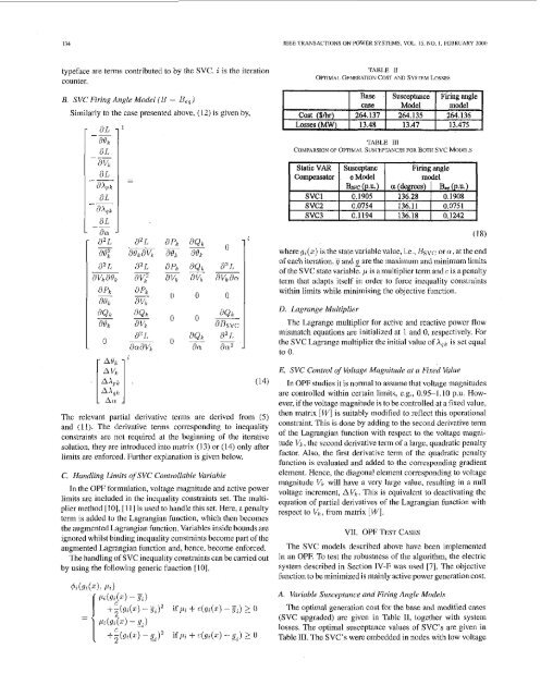A. Variable Susceptance and Firing Angle Models The optimal generation cost for the base and modified cases (SVC upgraded) are given in Table 11, together with system losses. The optimal susceptance values of SVC's are given in Table 111. The SVC's were embedded in nodes with low voltage
AMBRIZ-PBRBZ ADVANCED svc MODEIS FOR NEWTON-RAPHSON MAD FLOW AND NEWTON OPTIMAL POWER FLOW STUDIES 135 .- 2 " 1 300 - g 290 - .s 280 - + D t 270 - !? 2 260 - a SVC toto1 susceptanre model $ 250. SVCfiring ongle model ?. 4' 2 4 C L ' ' ' ' ' 0 1 2 3 4 5 6 34 1 32 - 30- YI 28- 26- 3 24- g 22- a 20. %! z 18- ' 16- 14 - lterotions Fig. 7. Active power generiltion cos1 pr~fil~s Fig. X. \ --- - Base case N C total susceptonce model . SVC iiring ongle model 1 2 5 r - 7 ' 1 " 3 " 4 " 5 ' 6 Iterations Active puwer lasses profiles. magnitudes and, as expected, the voltage profiles improved in such nodes (not shown). SVC voltage magnitudes were subjected to inequality constraints within 0.95-1.10 pa. In all cases, solutions were achieved in 6 iterations. Fig. 7 shows active power generation cost as a function of the iteration number whilst Fig. 8 shows the active power losses as a function of the iteration number. Oscillations can be observed in the cost and losses profiles in the early iterations. This is due to large variations in both the active set constraint and the penalty weighting factors during the early iterations. The SVC control specifications used above werc modified in order to assess the SVC inodcl capability to control voltage magnitude at fixed values. In this case the SVC's were set to control voltage magnitudes at I p.u. The optimal SVC state variable values for both models, i.c. susceptance and firing angle models, are shown in Table IV. As expected, these values difler from those given in Table 111. It is interesting to note that both SVC operating control modes, i.e. fixed and free, produce similar active power generation cost and active power losses. B. Transmission Lusses Minimization The algorithm is now applied to investigate the problem of transmission loss tniniinimtion. The active power cost optimization and the transmission losses minimization procedures TABLE 1V COMPARISON OmlMAL SUSCEPPANCE FOR BOTH SVC MODELS Firing angle 0.2150 136.32 0.2151 0.0741 136.10 0.0741 0.1376 136.20 0.1377 TABLE V OI'TIMAL GENERATION COST ANU SYSTEM LOSSES Base Susceptance Firingangle case Model model cost (Sib) 264.136 264.134 264.134 I7 475 11AKl 1.018L-12.23 1.021L-12.23 I I &40'00 6141.736 + Fig. 9. Comparison between the gewmov and susceptiince SVC ,nod& for the case when upp~ limits have bcen reached. are carried out sequentially. Transmission loss minimization is amenable to a redistribution of the reactive power throughout the network, which in turn induces changes in the active power generated by the slack generator. This may then result in an additional reduction of the active power generation cost. Table V presents results obtained with the combined optimization algorithm for the case when the SVC's are not set to maintain nodal voltage magnitude at a specified value. It can be observed that the second optimization exercise, i.e., network loss minimization, has only a minor effect on the active power generation cost. The network losses were reduced in only 0.15%, but a more uniform voltage profile was observed in all nodes (not shown). The reason for such a small variation in the network losses is due to the fact that the first optimization exercise, active power cost optimization, indirectly reduces the transmission network losses, i.e., large network losses means more active generation. The network loss minimization cases converged in 2 iterations C. Limitations of the Generator Model In order to show the limitations of the generator representation of an SVC, compared to the two SVC models introduced in this paper, a case is presented below where the SVC hits its upper reactive limit. SVC 1 was assumed to have a 40 MVAR upperlimit. Fig. 9 shows thereactive powers contributed by both models, where the network losses objective function was minimized. It can be observed that the reactive powers drawn by bath SVC models differ. The reason is that the reactive power is not really constant, as taken to be by the generator representation, but afunction of nodal voltage magnitude, as correctly indicated
Page 1 and 2: IEEE TRANSACTIONS ON POWER SYSTEMS.
Page 3 and 4: AMBRIZPkREZ ctnl.: ADVANCE0 SVC MOU
Page 5: AMRKIZPEREZ eta!.: ADVANCE0 SVC MOD

Advanced SVC models for newton-raphson load flow and ... - ITCJ

Create successful ePaper yourself

Delete template?

Save as template?