Introduction to Electrodynamics - HEP
Introduction to Electrodynamics - HEP
Introduction to Electrodynamics - HEP

Create successful ePaper yourself
Turn your PDF publications into a flip-book with our unique Google optimized e-Paper software.
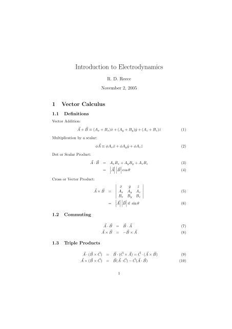
<strong>Introduction</strong> <strong>to</strong> <strong>Electrodynamics</strong><br />
R. D. Reece<br />
November 2, 2005<br />
1 Vec<strong>to</strong>r Calculus<br />
1.1 Definitions<br />
Vec<strong>to</strong>r Addition:<br />
Multiplication by a scalar:<br />
Dot or Scalar Product:<br />
⃗A + ⃗ B ≡ (A x + B x )ˆx + (A y + B y )ŷ + (A z + B z )ẑ (1)<br />
φ ⃗ A ≡ φA xˆx + φA y ŷ + φA z ẑ (2)<br />
⃗A · ⃗B = A x B x + A y B y + A z B z (3)<br />
= ∣A<br />
⃗ ∣ ∣B<br />
⃗ ∣ cos θ (4)<br />
Cross or Vec<strong>to</strong>r Product:<br />
⃗A × ⃗ B =<br />
=<br />
∣ ˆx ŷ ẑ ∣∣∣∣∣ A x A y A z<br />
(5)<br />
∣ B x B y B z ∣A<br />
⃗ ∣ ∣B<br />
⃗ ∣ ⃗n sin θ (6)<br />
1.2 Commuting<br />
⃗A · ⃗B = ⃗ B · ⃗A (7)<br />
⃗A × ⃗ B = − ⃗ B × ⃗ A (8)<br />
1.3 Triple Products<br />
⃗A · ( ⃗ B × ⃗ C) = ⃗ B · ( ⃗ C × ⃗ A) = ⃗ C · ( ⃗ A × ⃗ B) (9)<br />
⃗A × ( ⃗ B × ⃗ C) = ⃗ B( ⃗ A · ⃗C) − ⃗ C( ⃗ A · ⃗B) (10)<br />
1
1.4 Vec<strong>to</strong>r Derivatives in Cartesian Coordinates<br />
Gradient:<br />
Divergence:<br />
Curl:<br />
Laplacian of a scalar:<br />
Laplacian of a vec<strong>to</strong>r:<br />
1.5 Product Rules<br />
∇φ = ∂φ ∂φ ˆx +<br />
∂x ∂y ŷ + ∂φ<br />
∂z ẑ (11)<br />
∇ · ⃗v = ∂⃗v<br />
∂x + ∂⃗v<br />
∂y + ∂⃗v<br />
∂z<br />
(12)<br />
∣ ˆx ŷ ẑ ∣∣∣∣∣<br />
∇ × ⃗v =<br />
∂ ∂ ∂<br />
∂x ∂y ∂z<br />
(13)<br />
∣ v x v y v z<br />
∇ 2 φ ≡ ∇ · ∇φ (14)<br />
= ∂2 φ<br />
∂x 2 + ∂2 φ<br />
∂y 2 + ∂2 φ<br />
∂z 2 (15)<br />
∇ 2 ⃗v = ˆx∇ 2 v x + ŷ∇ 2 v y + ẑ∇ 2 v z (16)<br />
∇(fg) = f(∇g) + g(∇f) (17)<br />
∇( ⃗ A · ⃗B) = ⃗ A × (∇ × ⃗ B) + ⃗ B × (∇ × ⃗ A) + ( ⃗ A · ∇) ⃗ B + ( ⃗ B · ∇) ⃗ A(18)<br />
∇ · (f ⃗ A) = f(∇ · ⃗A) + ⃗ A · (∇f) (19)<br />
∇ · ( ⃗ A × ⃗ B) = ⃗ B · (∇ × ⃗ A) − ⃗ A · (∇ × ⃗ B) (20)<br />
∇ × (f ⃗ A) = (21)<br />
∇ × ( ⃗ A × ⃗ B) = (22)<br />
1.6 Second Derivatives<br />
1.7 Vec<strong>to</strong>r Implications<br />
1.8 Taylor’s Theorem<br />
For f : R → R:<br />
f(x 0 + x) =<br />
∞∑<br />
k=0<br />
f (k) (x 0 )<br />
x k =<br />
k!<br />
k=0<br />
∞∑<br />
k=0<br />
1<br />
k!<br />
d k f(x)<br />
dx k ∣<br />
∣∣∣x=x0<br />
x k (23)<br />
For f : R n → R, in vec<strong>to</strong>r notation:<br />
∞∑ 1<br />
f(⃗r 0 + ⃗r) =<br />
k! (⃗r · ∇| ⃗r= ⃗r 0<br />
) k f(⃗r) (24)<br />
2
1.9 Fundamental Theorems<br />
The Fundamental Theorem of Calculus:<br />
∫ b<br />
The Fundamental Theorem of Gradients:<br />
∫ ⃗a<br />
a<br />
df<br />
dx = f(b) − f(a) (25)<br />
dx<br />
⃗ b<br />
∇f(⃗r) · d ⃗ l = f( ⃗ b) − f(⃗a) (26)<br />
S<strong>to</strong>kes’ Theorem or The Curl Theorem:<br />
∫<br />
∮<br />
∇ × f(⃗r) ⃗ · dS ⃗ =<br />
⃗f(⃗r) · d ⃗ l (27)<br />
Gauss’ Theorem or The Divergence Theorem:<br />
∫<br />
∮<br />
∇ · ⃗f(⃗r) dV = ⃗f(⃗r) · dS ⃗ (28)<br />
Generalized S<strong>to</strong>kes’ Theorem:<br />
∫ ∫<br />
df = f (29)<br />
m ∂m<br />
1.10 The Laplacian<br />
The Laplacian opera<strong>to</strong>r acting on a scalar φ is denoted and defined as:<br />
∇ 2 φ ≡ ∇ · ∇φ (30)<br />
which reduces <strong>to</strong> following in R n :<br />
∇ 2 φ =<br />
n∑<br />
k=0<br />
∂ 2 φ<br />
∂x 2 k<br />
(31)<br />
in R 3 :<br />
∇ 2 φ = ∂2 φ<br />
∂x 2 + ∂2 φ<br />
∂y 2 + ∂2 φ<br />
∂z 2 (32)<br />
To demonstrate demonstrate what the Laplacian means, consider the average<br />
value of φ in a cube centered at the origin and with sides of length a,<br />
〈φ〉 = 1 V<br />
Taylor expanding φ gives:<br />
[<br />
φ = φ 0 + x ∂φ<br />
∂x + y ∂φ<br />
∂y + z ∂φ ]<br />
∂z<br />
∫<br />
φ dV = 1 ∫∫∫ a/2<br />
a 3 φ dx dy dz (33)<br />
−a/2<br />
φ=φ 0<br />
3
+ 1 [<br />
]<br />
x 2 ∂2 φ<br />
2 ∂x 2 + y2 ∂2 φ<br />
∂y 2 + z2 ∂2 φ<br />
∂z 2 + 2xy ∂2 φ<br />
∂x∂y + 2xz ∂2 φ<br />
∂x∂z + 2yz ∂2 φ<br />
+ ...<br />
∂y∂z<br />
φ=φ 0<br />
(34)<br />
After plugging this expansion in<strong>to</strong> the volume integral, all of the terms give zero<br />
when integrated except for φ 0 and the quadratic terms.<br />
〈φ〉 ≈ 1 ∫∫∫ (<br />
a/2<br />
a 3 φ 0 + 1 [<br />
] )<br />
x 2 ∂2 φ<br />
−a/2 2 ∂x 2 + y2 ∂2 φ<br />
∂y 2 + z2 ∂2 φ<br />
∂z 2 dx dy dz (35)<br />
φ=φ 0<br />
〈φ〉 ≈ 1 (<br />
a 3 a 3 φ 0 + a5<br />
24 ∇2 φ ∣ )<br />
φ=φ0<br />
(36)<br />
∇ 2 φ ∣ ∣<br />
φ=φ0<br />
≈ 24<br />
a 2 (〈φ〉 − φ 0) (37)<br />
This approximation gets more accurate as the volume considered for the average<br />
gets smaller. This demonstrates that the Laplacian is a measure of the difference<br />
between the value of the function at the point evaluated and the average value of<br />
the function in a region near that point.<br />
2 Maxwell’s Equations<br />
2.1 Gauss’ Law<br />
∇ · ⃗E = ρ ɛ 0<br />
(38)<br />
The divergence of the electric field is proportional <strong>to</strong> the charge density at that<br />
point. This means that charge is the source of the electric field. Integrating<br />
over a volume and applying Gauss’ Theorem <strong>to</strong> Gauss’ Law gives:<br />
∫<br />
∫<br />
∇ · ⃗E ρ<br />
dV = dV (39)<br />
ɛ<br />
∮<br />
0<br />
⃗E · dS ⃗ = Q (40)<br />
ɛ 0<br />
Where Q is the charge enclosed by the surface S. Above is the integral form of<br />
Gauss’ Law. It shows that the flux of the electric field over a closed surface is<br />
proportional <strong>to</strong> the charge enclosed by that surface.<br />
2.2 Divergence of the Magnetic Field<br />
∇ · ⃗B = 0 (41)<br />
The divergence of the magnetic field is zero, meaning there are no magnetic<br />
monopoles, no sources where the field lines begin or end like the charges for the<br />
electric field. Integrating over a volume and applying Gauss’ Theorem gives:<br />
∫<br />
∫<br />
∇ · ⃗B dV = 0 dV (42)<br />
∮<br />
⃗B · dS ⃗ = 0 (43)<br />
4
This integral form shows that the net flux of the magnetic field through a closed<br />
surface is always zero. Every field line that comes in must also leave.<br />
2.3 Faraday’s Law<br />
∇ × E ⃗ = − ∂ B ⃗ (44)<br />
∂t<br />
Integrating over a surface and applying S<strong>to</strong>kes’ Theorem gives:<br />
∫<br />
∫<br />
∇ × E ⃗ · dS ⃗ ∂B<br />
⃗<br />
= −<br />
∂t · d⃗ S (45)<br />
∮<br />
⃗E · d ⃗ l = − d ∫<br />
⃗B · dS dt<br />
⃗ (46)<br />
Faraday’s Law describes how a change in magnetic flux induces an electric field<br />
on the boundary of the surface considered for the flux. The negative sign in<br />
Faraday’s law is a consequence of Lenz’s Law which states that: the induced<br />
electric field is oriented in such a way as <strong>to</strong> induce a magnetic field which opposes<br />
the change in magnetic flux.<br />
2.4 Ampere’s Law<br />
∇ × B ⃗ ∂E<br />
= µ 0<br />
⃗j + µ 0 ɛ ⃗ 0 (47)<br />
∂t<br />
Integrating over a surface and applying S<strong>to</strong>kes’ Theorem gives:<br />
∫<br />
∫ (<br />
∇ × B ⃗ · dS ⃗ ∂<br />
= µ 0<br />
⃗j + µ 0 ɛ ⃗ )<br />
E<br />
0 · dS ∂t<br />
⃗ (48)<br />
∮<br />
∫<br />
⃗B · d ⃗ l = µ 0I ⃗<br />
d + µ0 ɛ 0<br />
⃗E · dS dt<br />
⃗ (49)<br />
Ampere’s Law describes how either currents, or a change in electric flux induces<br />
a magnetic field. The first term, µ 0I, ⃗ in Ampere’s Law show’s how a current<br />
induces a magnetic field that curls around that current according <strong>to</strong> the righthand-rule.<br />
The second term shows how a change of electric field in free space<br />
creates a magnetic field curling along the boundary of the surface considered for<br />
∂E<br />
electric flux. The quantity ɛ ⃗ 0 ∂t<br />
is called the displacement current, even though<br />
it is not a real current. In current carrying wires, the displacement current<br />
term is usually negligible compared <strong>to</strong> the first term because the displacement<br />
current includes the very small constant ɛ 0 in addition <strong>to</strong> µ 0 . We will see later<br />
that this second term is essential <strong>to</strong> the propagation of light.<br />
2.5 Summary<br />
One can divide Maxwell’s equations in<strong>to</strong> two pairs of equations: the divergence<br />
equations and the curl equations. The divergence equations tell what the static<br />
5
sources of the electric and magnetic fields are. The electric field is emitted from<br />
charges, while the magnetic field has no static source.<br />
The curl equations describe how the electric and magnetic fields can be<br />
induced— created by the dynamics of another field (or current) and not from a<br />
static source charge. The induced field is the curled field in each equation with<br />
the source of induction on the right side of each equation.<br />
Maxwell’s equations collected in their entirety:<br />
3 Electrostatics<br />
∇ · ⃗E = ρ ɛ 0<br />
(50)<br />
∇ · ⃗B = 0 (51)<br />
∇ × ⃗ E = − ∂ ⃗ B<br />
∂t<br />
∇ × ⃗ B = µ 0<br />
⃗j + µ 0 ɛ 0<br />
∂ ⃗ E<br />
∂t<br />
3.1 Time-Independent Electric Scalar Potential<br />
(52)<br />
(53)<br />
Charge densities constant in time ⇒ electric fields are constant in time; the<br />
theory of which is called electrostatics. Steady currents ⇒ magnetic fields are<br />
constant in time; the theory of which is called magne<strong>to</strong>statics.<br />
In the static senerio, we notice from Faraday’s Law that ∇ × ⃗ E = 0. This<br />
fact can tell us something very unique about the static electric field. It follows<br />
from S<strong>to</strong>kes’ Theorem that ∮ ⃗ E · d ⃗ l = 0. That is, any line integral of the electric<br />
field around a closed path gives zero. I can break a closed path in<strong>to</strong> two paths<br />
and vary one of them while keeping its end points so that the two paths still<br />
make a closed loop. The line integral of the electric field has <strong>to</strong> give zero on<br />
this augmented path also. Thus the augmented path must have the same line<br />
integral of the electric field as the original path. In electrostatics, the line integral<br />
of the electric field only depends on the end points of the path. Because of this,<br />
⃗E is called a conservative field. In general, the criterion for a field, ⃗ f, <strong>to</strong> be<br />
conservative is ∇ × ⃗ f = 0.<br />
Because the line integral of the electric field is independent of path, we can<br />
define a function, φ, called the electric potential:<br />
∫ ⃗r<br />
φ(⃗r) ≡ − ⃗E · d ⃗ l (54)<br />
⃗o<br />
Where ⃗o is the reference point taken <strong>to</strong> be zero potential. The potential difference<br />
between two points ⃗ b and ⃗a is:<br />
∫ ⃗ b ∫ ⃗a<br />
φ( ⃗ b) − φ(⃗a) = − ⃗E · d ⃗ l + ⃗E · d ⃗ l (55)<br />
⃗o<br />
⃗o<br />
6
∫ ⃗ b<br />
= −<br />
= −<br />
⃗o<br />
∫ ⃗ b<br />
⃗a<br />
∫ ⃗o<br />
⃗E · d ⃗ l − ⃗E · d ⃗ l (56)<br />
⃗a<br />
⃗E · d ⃗ l (57)<br />
Which corresponds <strong>to</strong> the fundamental theorem of gradients that:<br />
φ( ⃗ b) − φ(⃗a) =<br />
∫ ⃗ b<br />
Because this is true for any ⃗a and ⃗ b, it must be that:<br />
⃗a<br />
∇φ · d ⃗ l (58)<br />
⃗E = −∇φ (59)<br />
The fundamental theorem of gradients brings <strong>to</strong> light the fact that the path<br />
integral of the electric field only depends on the end points because the electric<br />
field can be written as the gradient of some scalar function. The electric potential<br />
is a continuous scalar function in space and the electric field points in the<br />
direction of steepest descent of electric potential. One can also see that writing<br />
the electric field as ⃗ E = −∇φ satisfies the electrostatic case that ∇ × ⃗ E = 0<br />
because the ∇ × ∇f = 0 for any scalar function f.<br />
3.2 Poisson’s Equation<br />
Writing Gauss’ Law with ⃗ E = −∇φ gives:<br />
−∇ · ∇φ = −∇ 2 φ = ρ ɛ 0<br />
(60)<br />
∇ 2 φ = − ρ ɛ 0<br />
(61)<br />
This equation has the form known as Poisson’s Equation:<br />
∇ 2 u = v (62)<br />
With the condition that u → 0 as r → ∞, it has the solution:<br />
u(⃗r) = −1 ∫<br />
v(⃗r ′ )<br />
∣<br />
4π ∣ ∣∣<br />
d 3 r ′ (63)<br />
∣⃗r − ⃗r ′<br />
Therefore the solution <strong>to</strong> our Poisson’s equation of φ with ∞ chosen <strong>to</strong> be our<br />
reference point where φ(∞) = 0 is:<br />
φ(⃗r) = 1 ∫<br />
ρ(⃗r ′ )<br />
∣<br />
4πɛ 0<br />
∣ ∣∣<br />
d 3 r ′ (64)<br />
∣⃗r − ⃗r ′<br />
This is a formal solution <strong>to</strong> Poisson’s Equation. In the context of a problem,<br />
this integral is usually difficult <strong>to</strong> solve. Later, there is a discussion of more<br />
applicable ways <strong>to</strong> solve Poisson’s Equation.<br />
7
3.3 Coulomb’s Law<br />
Taking minus the gradient of our solution for the electric scalar potential should<br />
give us a general soultion for the electric field for a given charge distribution, ρ.<br />
⃗E(⃗r) = −∇φ(⃗r) (65)<br />
⎛ ⎞<br />
= −1 ∫<br />
ρ(⃗r<br />
4πɛ ′ )∇ ⎝ 1 ∣⎠ 0<br />
∣ ∣∣<br />
d 3 r ′ (66)<br />
∣⃗r − ⃗r ′<br />
)<br />
∫<br />
1 ρ( ⃗r ′ )<br />
(⃗r − ⃗r ′<br />
=<br />
∣<br />
4πɛ 0 ∣ ∣∣<br />
∣⃗r − ⃗r ′ 3<br />
d 3 r ′ (67)<br />
This is known as Coulomb’s Law: that the electric field at position ⃗r generated<br />
by a single particle with charge q at position ⃗r ′ is:<br />
)<br />
⃗E(⃗r) = 1 q<br />
(⃗r − ⃗r ′ ∣<br />
4πɛ 0 ∣ ∣∣<br />
∣⃗r − ⃗r ′ 3<br />
(68)<br />
Therefore, an assortment n of particles creates a field:<br />
⃗E(⃗r) = 1 ∑<br />
n q i<br />
(⃗r − ⃗ )<br />
r i<br />
′ 4πɛ 0 ∣<br />
i=1 ∣⃗r − r ⃗ i<br />
′ ∣ 3 (69)<br />
If the charge distribution is continuous instead of discrete, the sum becomes an<br />
integral over all space:<br />
)<br />
⃗E(⃗r) = 1 ∫ ρ( ⃗r ′ )<br />
(⃗r − ⃗r ′ ∣<br />
4πɛ 0 ∣ ∣∣<br />
∣⃗r − ⃗r ′ 3<br />
d 3 r ′ (70)<br />
The primary importance of fields is that they can be used <strong>to</strong> determine the<br />
force on a particle. The relation between a force ⃗ F on a particle with charge Q<br />
and the electric field E is:<br />
⃗F = Q ⃗ E (71)<br />
The advantage that taking the intemediate step of calculating the scalar potential<br />
instead of calculating the electric field directly with Coulomb’s law is that<br />
the integral used <strong>to</strong> calculate the scalar potential is of a scalar quantity while<br />
Coulomb’s law uses vec<strong>to</strong>rs. Calculating the scalar potential does not require<br />
the consideration of components. The electric field can easily be determined by<br />
taking minus the gradient of the scalar potential.<br />
8
3.4 Electrostatic Energy<br />
3.5 Conduc<strong>to</strong>rs<br />
3.6 Boundary Conditions of the Electric Field<br />
3.7 Capaci<strong>to</strong>rs<br />
3.8 The Uniqueness Theorem<br />
3.9 Methods of Solving Poisson’s Equation<br />
3.9.1 Method of Images<br />
3.9.2 Method of Complex Analysis<br />
3.9.3 Method of Seperation of Variables<br />
4 Magne<strong>to</strong>statics<br />
9