Gr 10 Data Handling 3 - Maths Excellence
Gr 10 Data Handling 3 - Maths Excellence
Gr 10 Data Handling 3 - Maths Excellence

Create successful ePaper yourself
Turn your PDF publications into a flip-book with our unique Google optimized e-Paper software.
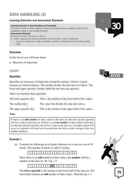
DATA HANDLING (3)<br />
Learning Outcomes and Assessment Standards<br />
Learning Outcome 4: <strong>Data</strong> <strong>Handling</strong> and Probability<br />
The learner is able to collect, organise, analyse and interpret data to establish statistical and<br />
probability models to solve related problems.<br />
Assessment Standards<br />
We know this when the learner is able to:<br />
• Collect, organise and interpret univariate numerical data in order to determine:<br />
◦ measures of dispersion: range, percentiles, quartiles, interquartile and semi-inter-quartile<br />
range.<br />
Lesson 30<br />
Overview<br />
In this lesson you will learn about:<br />
●<br />
Measures of dispersion.<br />
Lesson<br />
Quartiles<br />
Quartiles are measures of dispersion around the median, which is a good<br />
measure of central tendency. The median divides the data into two halves. The<br />
lower and upper quartiles further subdivide the data into quarters.<br />
There are therefore three quartiles:<br />
The lower quartile (Q 1<br />
):<br />
The median (Q 2<br />
):<br />
The upper quartile (Q 3<br />
):<br />
Note:<br />
This is the median of the lower half of the values.<br />
The value that divides the data into halves.<br />
This is the median of the upper half of the values.<br />
DVD<br />
If there is an odd number of data values in the data set, then the specific quartile<br />
will be a value in the data set. If there is an even number of data values in the data<br />
set then the specific quartile will not be a value in the data set. A number which will<br />
serve as a quartile will need to be inserted into the data set (the average of the two<br />
middle numbers).<br />
Example 1<br />
(a) Consider the following set of marks obtained on a class test out of <strong>10</strong><br />
marks. The number of marks is odd (11 marks).<br />
2 2 3 4 5 5 6 7 7 8 9<br />
Since there is an odd number of data values, the median will be a<br />
number in the data set. M = Q 2<br />
= 5.<br />
2 2 3 4 5 5 6 7 7 8 9<br />
The lower quartile is the median of the lower half of the data set. The<br />
lower half contains an odd number of data values. Therefore Q 1<br />
= 3.<br />
15<br />
<strong>10</strong> LC G<strong>10</strong> MATHS LWB.indb 15 2008/09/09 12:22:42 PM
In summary:<br />
2 2 3 4 5<br />
The upper quartile is the median of the upper half of the data set.<br />
The upper half contains an odd number of data values.<br />
Therefore Q 2<br />
= 7.<br />
6 7 7 8 9<br />
2 2 3 4 5 5 6 7 7 8 9<br />
Lower Quartile<br />
Q 1<br />
Median<br />
Q 2<br />
Upper Quartile<br />
Q 3<br />
(b) Consider the following set of 13 marks obtained on a class test out of<br />
<strong>10</strong> marks:<br />
2 3 4 5 5 5 6 7 7 8 8 <strong>10</strong> <strong>10</strong><br />
Since there is an odd number of data values, the median will a number in<br />
the data set. M = Q 2<br />
= 6.<br />
2 3 4 5 5 5 6 7 7 8 8 <strong>10</strong> <strong>10</strong><br />
The lower quartile is the median of the lower half of the data set. The<br />
lower half contains an even number of data values. Therefore we need to<br />
find the average of the two middle numbers, 4 and 5 and then insert this<br />
number into the data set:<br />
Q 1<br />
= _ 4 + 5 = 4,5<br />
2<br />
Q 1<br />
2 3 4 4,5 5 5 5<br />
The upper quartile is the median of the upper half of the data set. The<br />
upper half contains an even number of data values. Therefore we need to<br />
find the average of the two middle numbers, 8 and 8 and then insert this<br />
number into the data set:<br />
Q 3<br />
= _ 8 + 8 = 8<br />
2<br />
Q 3<br />
7 7 8 8 8 <strong>10</strong> <strong>10</strong><br />
In summary:<br />
2 3 4 4,5 5 5 5 6 7 7 8 8 8 <strong>10</strong> <strong>10</strong><br />
Q 1<br />
Q 2<br />
Q 3<br />
Example 2<br />
(a) Consider the following set of 12 marks obtained by a class on a class<br />
test out of <strong>10</strong>0 marks. The number of marks is even.<br />
20 32 43 54 55 61 73 78 89 90 91 98<br />
16<br />
<strong>10</strong> LC G<strong>10</strong> MATHS LWB.indb 16 2008/09/09 12:22:43 PM
Since there is an even number of data values, the median will not be a data<br />
value in the data set. We will need to find the average of the two middle<br />
numbers, 61 and 73 and then insert this number into the data set:<br />
61 + 73<br />
M = Q 2<br />
= _ = 67<br />
2<br />
20 32 43 54 55 61 67 73 78 89 90 91 98<br />
The lower quartile is the median of the lower half of the data set. The<br />
lower half contains an even number of data values. Therefore we need to<br />
find the average of the two middle numbers, 43 and 54 and then insert this<br />
number into the data set:<br />
43 +54<br />
Q 1<br />
= _ = 48,5<br />
2<br />
Q 1<br />
20 32 43 48,5 54 55 61<br />
The upper quartile is the median of the upper half of the data set. The<br />
upper half contains an even number of data values. Therefore we need to<br />
find the average of the two middle numbers, 89 and 90 and then insert this<br />
number into the data set:<br />
89 + 90<br />
Q 3<br />
= _ = 89,5<br />
2<br />
Q 3<br />
73 78 89 89,5 90 91 98<br />
In summary:<br />
20 32 43 48,5 54 55 61 67 73 78 89 89,5 90 91 98<br />
(b) Consider the following set of <strong>10</strong> marks obtained by a class on a class<br />
test out of 150 marks. The number of marks is even.<br />
12 60 95 <strong>10</strong>5 120 125 130 135 140 142<br />
Since there is an even number of data values, the median will not be a data<br />
value in the data set. We will need to find the average of the two middle<br />
numbers, 120 and 125 and then insert this number into the data set:<br />
120 +125<br />
M = Q 2<br />
= __ = 122,5<br />
2<br />
12 60 95 <strong>10</strong>5 120 122,5 125 130 135 140 142<br />
The lower quartile is the median of the lower half of the data set. The<br />
lower half contains an odd number of data values. Therefore Q 1<br />
= 95.<br />
12 60 95 <strong>10</strong>5 120<br />
The upper quartile is the median of the upper half of the data set. The<br />
upper half contains an odd number of data values. Therefore Q 2<br />
= 135.<br />
125 130 135 140 142<br />
In summary:<br />
12 60 95 <strong>10</strong>5 120 122,5 125 130 135 140 142<br />
17<br />
<strong>10</strong> LC G<strong>10</strong> MATHS LWB.indb 17 2008/09/09 12:22:44 PM
INDIVIDUAL<br />
FORMATIVE<br />
ASSESSMENT<br />
Activity 1<br />
1. For each set of data, determine the quartiles:<br />
A 2 3 5 7 9 <strong>10</strong> 11 13 15 16 16 17 18 19 21 22 23 25 32<br />
B 2 3 5 7 9 <strong>10</strong> 11 13 15 16 16 17 18 19 21 22 23<br />
C 2 3 5 7 9 <strong>10</strong> 11 13 15 16 16 17 18 19 21 22 23 25 32 34<br />
D 2 3 5 7 9 <strong>10</strong> 11 13 15 16 16 17 18 19 21 22 23 25<br />
DVD<br />
Lesson<br />
Range<br />
The range is the difference between the largest and the smallest value in the<br />
data. The bigger the range, the more spread out the data is. The range cannot<br />
be used with grouped data and it doesn’t deal with values between these<br />
extremes. Also, a single very small or very large value would give a misleading<br />
impression of the spread of the data.<br />
Consider for example, the following set of marks for Class A:<br />
Class A 1 1 2 2 3 4 4 5 5 6 7 8 8 9 <strong>10</strong><br />
Range = largest score – smallest score = <strong>10</strong> – 1 = 9<br />
Deciles and percentiles<br />
Deciles subdivide the data into tenths. Percentiles divide the data into<br />
hundredths.<br />
The interquartile range (IQR)<br />
The difference between the lower and upper quartile is called the interquartile<br />
range. It is a better measure of dispersion than the range because it is not<br />
affected by extreme values. It is based on the middle half of the data. It<br />
indicates how densely the data in the middle is spread around the median.<br />
Example<br />
Calculate the interquartile range for the following data set.<br />
2 2 3 4 5 5 6 7 7 8 9<br />
Lower<br />
Quartile<br />
Q 1<br />
IQR = Q 3<br />
– Q 1<br />
= 7 – 3 = 4<br />
The semi-interquartile range<br />
Median<br />
Q 2<br />
Upper<br />
Quartile<br />
Q 3<br />
The semi-interquartile range is half of the interquartile range.<br />
The semi-IQR for the previous example is _<br />
Q – Q 3 1<br />
2<br />
= _ 7 – 3 = 2.<br />
2<br />
18<br />
<strong>10</strong> LC G<strong>10</strong> MATHS LWB.indb 18 2008/09/09 12:22:45 PM
Activity 2<br />
1. Class results for a test out of 30 are recorded in the table below.<br />
<strong>10</strong>A 16 12 16 11 14 15 22 16 17 15 26 23 16 22 16 17 24 19 16 -<br />
<strong>10</strong>B 20 19 14 <strong>10</strong> 14 9 8 13 14 30 27 23 24 28 17 29 20 16 14 18<br />
<strong>10</strong>C 5 20 14 12 7 2 12 21 14 26 14 14 12 14 21 24 14 14 - -<br />
INDIVIDUAL<br />
SUMMATIVE<br />
ASSESSMENT<br />
(a) Calculate the mean for each class.<br />
(b) Calculate the mode for each class.<br />
(c) Calculate the median for each class.<br />
(d) Calculate the range for each class.<br />
(e) Calculate the lower quartile for each class.<br />
(f) Calculate the upper quartile for each class.<br />
(g) Calculate the interquartile range for each class.<br />
(h) Calculate the semi-interquartile range for each class.<br />
2. Over a period of 15 days, the owner of a coffee shop recorded the number<br />
of customers who per day ordered the breakfast special. His observations<br />
were as follows:<br />
Day 1 2 3 4 5 6 7 8 9 <strong>10</strong> 11 12 13 14 15<br />
Number of orders 25 80 34 26 21 65 28 21 39 21 30 34 21 28 40<br />
Determine:<br />
(a) the mean<br />
(b) the median<br />
(c) the mode<br />
(d) the range<br />
(e) the inter-quartile range.<br />
(f) Which of the mean, median or mode is the most appropriate value in<br />
estimating how many orders will be made per day? Explain.<br />
19<br />
<strong>10</strong> LC G<strong>10</strong> MATHS LWB.indb 19 2008/09/09 12:22:46 PM
ANSWERS AND ASSESSMENT<br />
Lesson 28<br />
Activity 1<br />
1. (a)<br />
600<br />
500<br />
400<br />
300<br />
200<br />
<strong>10</strong>0<br />
0<br />
97/98 98/99 99/00 00/01 01/02 02/03 03/04 04/05 05/06 06/07 07/08<br />
(b) Inflation and increased population has caused the amounts to increase.<br />
2. Marks (<strong>10</strong>) Tally Frequency (f)<br />
1 || 2<br />
2 ||| 3<br />
3 ||| 4<br />
4 |||| | 6<br />
5 |||| 5<br />
6 |||| |||| 9<br />
7 ||| 3<br />
8 ||| 3<br />
9 || 2<br />
<strong>10</strong> ||| 3<br />
Total: 40<br />
20<br />
<strong>10</strong><br />
9<br />
8<br />
7<br />
6<br />
5<br />
4<br />
3<br />
2<br />
1<br />
0<br />
1 2 3 4 5 6 7 8 9 <strong>10</strong><br />
<strong>10</strong> LC G<strong>10</strong> MATHS LWB.indb 20 2008/09/09 12:22:48 PM
Mass<br />
3. Salaries R2 000 000<br />
<strong>Gr</strong>ounds and maintenance R 800 000<br />
Textbooks R 200 000<br />
Photocopying facilities R1 000 000<br />
Sporting facilities R 500 000<br />
Water and lights R 300 000<br />
Academic subject allocation R 200 000<br />
Computer centre R 700 000<br />
Administration R 200 000<br />
Salaries:<br />
<strong>Gr</strong>ounds and Maintenance:<br />
Textbooks:<br />
Photocopying:<br />
Sport:<br />
Water and lights<br />
Academic:<br />
Computer:<br />
Administration:<br />
2 __ 000 000<br />
× 360° = 122°<br />
5 900 000<br />
__ 800 000<br />
× 360° = 49°<br />
5 900 000<br />
__ 200 000<br />
× 360° = 12°<br />
5 900 000<br />
1 __ 000 000<br />
× 360° = 61°<br />
5 900 000<br />
__ 500 000<br />
× 360° = 31°<br />
5 900 000<br />
__ 300 000<br />
× 360° = 18°<br />
5 900 000<br />
__ 200 000<br />
× 360° = 12°<br />
5 900 000<br />
__ 700 000<br />
× 360° = 43°<br />
5 900 000<br />
__ 200 000<br />
× 360° = 12°<br />
5 900 000<br />
Academic<br />
Water and lights<br />
Computers<br />
Admin<br />
Sport<br />
Photocopying<br />
Salaries<br />
Textbooks<br />
<strong>Gr</strong>ounds<br />
4. (a)<br />
3,2 .<br />
3,1<br />
3,0<br />
2,9<br />
2,8<br />
2,7<br />
2,6<br />
2,5<br />
2,4<br />
2,3<br />
2,2<br />
2,1<br />
0<br />
. .<br />
.<br />
.<br />
.<br />
1 2 3 4 5 6 7 8 9 <strong>10</strong><br />
Week<br />
.<br />
.<br />
.<br />
.<br />
21<br />
<strong>10</strong> LC G<strong>10</strong> MATHS LWB.indb 21 2008/09/09 12:22:49 PM
Frequency<br />
Frequency<br />
(b) 6 th week<br />
(c) Average mass =<br />
Activity 2<br />
__ 2,3 + 2,6<br />
= 2,5 kg<br />
2<br />
1. (a)<br />
200<br />
180<br />
160<br />
140<br />
120<br />
<strong>10</strong>0<br />
80<br />
60<br />
40<br />
20<br />
(b)<br />
2. (a)<br />
200<br />
180<br />
160<br />
140<br />
120<br />
<strong>10</strong>0<br />
80<br />
60<br />
40<br />
20<br />
0-1,9 2-3,9 4-5,9 6-7,9 8-9,9 <strong>10</strong>-11,9 12-13,9 14-15,9<br />
Duration<br />
0,95<br />
2,95<br />
.<br />
.<br />
4,95<br />
.<br />
6,95<br />
0-1,9 2-3,9 4-5,9 6-7,9 8-9,9 <strong>10</strong>-11,9 12-13,9 14-15,9<br />
Duration<br />
.<br />
8,95<br />
.<br />
<strong>10</strong>,95<br />
.<br />
12,95<br />
14,95<br />
2 4<br />
3 6 6 8<br />
4 2 2 3 7 8 8 8<br />
5 2 4 4 4 4 5 5 5 5 6 6 7 7 8 8 8 9 9<br />
6 0 1 1 1 1 2 2 3 3 3 4 4 4 4 4 4 5 5 5 6 6 6 8 8 8 8 8 9 9 9 9<br />
7 0 0 2 2 2 3 3 3 3 4 4 4 4 4 4 4 4 4 5 5 5 5 5 6 6 6 6 6 6 6 7 8 8 8 8 9 9<br />
8 0 0 1 2 2 2 2 2 2 2 4 4 4 4 4 4 5 5 6 6 6 6 6 6 6 6 6 7 7 7 7 7 7 7 7 7 7 7 7 8 8 9 9 9 9 9 9 9<br />
9 0 0 0 1 1 4 4 4 5 5 5 5 6<br />
22<br />
<strong>10</strong> LC G<strong>10</strong> MATHS LWB.indb 22 2008/09/09 12:22:49 PM
Frequency<br />
Frequency<br />
(b) Class interval Frequency (number of clients per mass group)<br />
<strong>10</strong> – 19 kg 0<br />
20 – 29 kg 1<br />
30 – 39 kg 3<br />
40 – 49 kg 7<br />
50 – 59 kg 18<br />
60 – 69 kg 31<br />
70 – 79 kg 38<br />
80 – 89 kg 49<br />
90 – 99 kg 13<br />
<strong>10</strong>0 – <strong>10</strong>9kg 0<br />
(c)<br />
50<br />
40<br />
35<br />
30<br />
25<br />
20<br />
15<br />
<strong>10</strong><br />
5<br />
<strong>10</strong>-19 20-29 30-39 40-49 50-59 60-69 70-79 80-89<br />
Masses<br />
90-99 <strong>10</strong>0-<strong>10</strong>9<br />
(d)<br />
50<br />
40<br />
35<br />
30<br />
25<br />
20<br />
15<br />
<strong>10</strong><br />
5<br />
44,5<br />
34,5<br />
24,5<br />
14,5<br />
<strong>10</strong>-19 20-29 30-39 40-49 50-59 60-69 70-79 80-89<br />
Masses<br />
. .<br />
.<br />
.<br />
54,5<br />
.<br />
64,5<br />
.<br />
74,5<br />
.<br />
84,5<br />
.<br />
94,5<br />
<strong>10</strong>4,5<br />
90-99 <strong>10</strong>0-<strong>10</strong>9<br />
(e) The histogram shows that the majority of people were in the 80-89<br />
kg group. This group would probably either want to lose body fat<br />
and keep or gain muscle mass. It would be unlikely that this group<br />
would want to gain too much weight or lose too much. It seems that<br />
the health product company should market both products in Gauteng.<br />
The 50-69 kg group will benefit from the Muscle <strong>Gr</strong>ow product. The<br />
90-99 kg group will benefit from the Fat Go product.<br />
23<br />
<strong>10</strong> LC G<strong>10</strong> MATHS LWB.indb 23 2008/09/09 12:22:50 PM
Lesson 29<br />
Activity 1<br />
1. First arrange in ascending order.<br />
<strong>10</strong>A 11 12 14 15 15 16 16 16 16 16 16 17 17 19 22 22 23 24 26 -<br />
<strong>10</strong>B 8 9 <strong>10</strong> 13 14 14 14 14 16 17 18 19 20 20 23 24 27 28 29 30<br />
<strong>10</strong>C 2 5 7 12 12 12 14 14 14 14 14 14 14 20 21 21 24 26 - -<br />
333<br />
(a) Mean for <strong>10</strong>A: _<br />
19 = 17,5<br />
367<br />
Mean for <strong>10</strong>B: _<br />
20 = 18,4<br />
260<br />
Mean for <strong>10</strong>C: _<br />
18 = 14,4<br />
(b) Mode for <strong>10</strong>A: 16<br />
Mode for <strong>10</strong>B: 14<br />
Mode for <strong>10</strong>C: 14<br />
(c) Median for <strong>10</strong>A: 16<br />
Median for <strong>10</strong>B: 17,5<br />
Median for <strong>10</strong>C: 14<br />
2 4<br />
3 6 6<br />
4 2 2<br />
5 2 4<br />
6 0 1<br />
7 0 0<br />
8 0 0<br />
9 0 0<br />
2. (a) Marks (<strong>10</strong>) Tally Frequency (f) Mark × f<br />
Activity 2<br />
Discussion<br />
Activity 3<br />
1 || 2 2<br />
2 |||| 4 8<br />
3 |||| 5 15<br />
4 |||| 4 16<br />
5 | 1 5<br />
6 |||| 4 24<br />
7 |||| |||| 9 63<br />
8 |||| 4 32<br />
9 |||| 4 36<br />
<strong>10</strong> ||| 3 30<br />
Total: 40 Total: 231<br />
Mean = _ 231 = 5,8 Mode = 7 Median = 5,5<br />
40<br />
1. (a) 6 – 7,9 interval.<br />
(b) 6 – 7,9 interval.<br />
24<br />
<strong>10</strong> LC G<strong>10</strong> MATHS LWB.indb 24 2008/09/09 12:22:51 PM
2. (a)<br />
4<br />
6 6 8<br />
2 2 3 7 8 8 8<br />
2 4 4 4 4 5 5 5 5 6 6 7 7 8 8 8 9 9<br />
0 1 1 1 1 2 2 3 3 3 4 4 4 4 4 4 5 5 5 6 6 6 8 8 8 8 8 9 9 9 9<br />
0 0 2 2 2 3 3 3 3 4 4 4 4 4 4 4 4 4 5 5 5 5 5 6 6 6 6 6 6 6 7 8 8 8 8 9 9<br />
0 0 1 2 2 2 2 2 2 2 4 4 4 4 4 4 5 5 6 6 6 6 6 6 6 6 6 7 7 7 7 7 7 7 7 7 7 7 7 8 8 9 9 9 9 9 9 9<br />
0 0 0 1 1 4 4 4 5 5 5 5 6<br />
(b)<br />
Class interval Frequency Midpoint class interval Frequency × Midpoint<br />
<strong>10</strong> – 19 kg – – –<br />
20 – 29 kg 1 24,5 24,5<br />
30 – 39 kg 3 34,5 <strong>10</strong>3,5<br />
40 – 49 kg 7 44,5 311,5<br />
50 – 59 kg 18 54,5 981<br />
60 – 69 kg 31 64,5 1999,5<br />
70 – 79 kg 38 74,5 2831<br />
80 – 89 kg 49 84,5 4140,5<br />
90 – 99 kg 13 94,5 1228,5<br />
<strong>10</strong>0 – <strong>10</strong>9kg - - -<br />
Totals 160 - 11620<br />
11 620<br />
(c) Estimated mean = _<br />
160 = 72,6<br />
Lesson 30<br />
Activity 1<br />
A 2 3 5 7 9 <strong>10</strong> 11 13 15 16 16 17 18 19 21 22 23 25 32<br />
B 2 3 5 7 8 9 <strong>10</strong> 11 13 15 16 16 17 18 18,5 19 21 22 23<br />
C 2 3 5 7 9 9,5 <strong>10</strong> 11 13 15 16 16 16 17 18 19 21 21,5 22 23 25 32 34<br />
D 2 3 5 7 9 <strong>10</strong> 11 13 15 15,5 16 16 17 18 19 21 22 23 25<br />
Activity 2<br />
333<br />
1. (a) Mean for <strong>10</strong>A: _<br />
19 = 17,5<br />
367<br />
Mean for <strong>10</strong>B: _<br />
20 = 18,4<br />
260<br />
Mean for <strong>10</strong>C: _<br />
18 = 14,4<br />
(b) Mode for <strong>10</strong>A: 16<br />
Mode for <strong>10</strong>B: 14<br />
Mode for <strong>10</strong>C: 14<br />
(c) Median for <strong>10</strong>A: 16<br />
Median for <strong>10</strong>B: 17,5<br />
Median for <strong>10</strong>C: 14<br />
25<br />
<strong>10</strong> LC G<strong>10</strong> MATHS LWB.indb 25 2008/09/09 12:22:52 PM
(d) Range for <strong>10</strong>A: 26 – 11 = 15<br />
Range for <strong>10</strong>B: 30 – 8 = 22<br />
Range for <strong>10</strong>C: 26 – 2 = 24<br />
(e) Lower quartile for <strong>10</strong>A: Q 1<br />
= 15<br />
Lower quartile for <strong>10</strong>B: Q 1<br />
= 14<br />
Lower quartile for <strong>10</strong>C: Q 1<br />
= 12<br />
(f) Upper quartile for <strong>10</strong>A: Q 3<br />
= 22<br />
Upper quartile for <strong>10</strong>B: Q 3<br />
= 23,5<br />
Upper quartile for <strong>10</strong>C: Q 3<br />
= 20,5<br />
(g) Interquartile range for <strong>10</strong>A: Q 3<br />
– Q 1<br />
= 22 – 15 = 7<br />
Interquartile range for <strong>10</strong>B: Q 3<br />
– Q 1<br />
= 23,5 – 14 = 9,5<br />
Interquartile range for <strong>10</strong>C: Q 3<br />
– Q 1<br />
= 20,5 – 12 = 8,5<br />
(h) Semi-interquartile range for <strong>10</strong>A: _<br />
Q – Q 3 1<br />
= _ 22 – 15<br />
= 3,5<br />
2 2<br />
Semi-interquartile range for <strong>10</strong>B: _<br />
Q – Q 3 1<br />
= __ 23,5 – 14<br />
= 4,75<br />
2 2<br />
Semi-interquartile range for <strong>10</strong>C: _<br />
Q – Q 3 1<br />
= __ 20,5 – 12<br />
= 4,25<br />
2 2<br />
2. (a) Mean = 34,2 orders<br />
(b) Median = 28 orders<br />
(c) Mode = 21 orders<br />
(d) Range = 80 – 21 = 59 orders<br />
(e) Interquartile range: Q 3<br />
– Q 1<br />
= 39 – 21 = 18<br />
(f) The mean would probably be the most accurate estimate. The mode<br />
and median are too small a number of orders per day. However, the<br />
owner would need to be prepared to make more than 34 orders on a<br />
few days, even up to 80!<br />
26<br />
<strong>10</strong> LC G<strong>10</strong> MATHS LWB.indb 26 2008/09/09 12:22:53 PM
TIPS FOR TEACHERS<br />
Lesson 28<br />
●<br />
●<br />
Ensure that learners know the difference between bar graphs and histograms.<br />
The points represented on a broken line graph should not be joined by means<br />
of a continuous solid line. This is because data values between these values<br />
are not known. The points should be joined by a dotted line.<br />
Reference<br />
“Mathematics textbook and workbook grade <strong>10</strong>”<br />
Allcopy publishers<br />
M.D.Phillips<br />
Lesson 29<br />
●<br />
Ensure that learners know that the median will be a number in the data if<br />
the number of data values is odd. If the number of data values is even, the<br />
median will be an insertion into the data set. In this case, the median will be<br />
the average between the two middle values.<br />
Reference<br />
“Mathematics textbook and workbook grade <strong>10</strong>”<br />
Allcopy publishers<br />
M.D.Phillips<br />
Lesson 30<br />
●<br />
●<br />
Ensure that learners know that the median will be a number in the data if<br />
the number of data values is odd. If the number of data values is even, the<br />
median will be an insertion into the data set. In this case, the median will be<br />
the average between the two middle values.<br />
The median is excluded from the lower and upper halves when determining<br />
the lower and upper quartiles.<br />
Reference<br />
“Mathematics textbook and workbook grade <strong>10</strong>”<br />
Allcopy publishers<br />
M.D.Phillips<br />
27<br />
<strong>10</strong> LC G<strong>10</strong> MATHS LWB.indb 27 2008/09/09 12:22:53 PM