Scatterer Characterisation Using Polarimetric SAR Tomography

Scatterer Characterisation Using
Polarimetric SAR Tomography
Stéphane Guillaso and Andreas Reigber
Berlin University of Technology, Computer Vision and Remote Sensing
Sekr. FR3-1, Franklinstr. 28/29, D-10587 Berlin, Germany
Email: stephane@cs.tu-berlin.de, anderl@cs.tu-berlin.de
Abstract— This paper presents the first step to characterise
scatterers using polarimetric SAR tomography (POLTOMSAR).
It is a logical extension of the tomographic data processing, which
consists to use the vectorial properties of electromagnetic waves.
An introduction to the estimation of the polarisation state of
retrieved target is proposed. It is based on a modified signal
model adapted to the MUSIC algorithm. This makes it possible
to determinate the physical nature of detected object, which is not
possible using classical approach, unless having the ground-truth
of the scene under study. The experimental results are shown
using a multibaseline data set acquired in L-band by DLR’s
experimental SAR (E-SAR) on a test site near Oberpfaffenhofen
/ Germany.
I. INTRODUCTION
SAR tomography is the extension of conventional twodimensional
SAR imaging principle to three dimensions. A
real three-dimensional imaging of a scene is achieved by
the formation of an additional synthetic aperture in elevation,
using a coherent combination of images acquired from several
parallel flight tracks. The introduction of tomographic SAR
offers the possibility of a direct localisation of all scattering
contributions in a volume [1], [2]. This greatly extends the
potential of SAR, particularly for the analysis of volume
structures, like for example forests or urban areas [3], [4].
Up to now, different investigation of high-resolution approaches,
like Capon [2], MUSIC [3], were proposed in
order to improve the resolution achieved using the standard
beamforming Fourier-based method [1]. These methods are
often employed for so-called DoA (Direction-of-Arrical) of
received waves using an antenna array. Basically, a multibaseline
acquisition sustem represents an antenna array and
these methods can be applied in order to determine the height
of dominant scatterers. there are presented in section II. All
these approaches make it possible to retrieve the position
of scatterers over volumetric areas, but give any information
about the nature of the scatterer itself unless having the
ground-truth of the scene under study.
A first approach to characterise the nature of retrieved target
is presented in section III. It is based on a modified signal
model adapted to MUSIC algorithm. This approach is applied
to partial polarimetric data [3]. On the one hand, the MUSIC
approach is able to give a higher precision about the scatterer
height than using only single channel SAR data. On the
other hand, polarimetric MUSIC approach makes it possible to
0-7803-9051-2/05/$20.00 (C) 2005 IEEE
retrieve a partial polarimetric characterisation of the scatterer
observed.
The efficiency of this polarimetric SAR tomography analysis
is demonstrated using 14 fully polarimetric SAR images,
obtained from DLR-ESAR airborne sensor in L-band repeatpass
mode.
II. MONOCHANNEL SAR TOMOGRAPHY
L
x
z
n
r
1
2 ···
K − 1
K
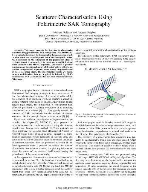
Fig. 1. Principle of multibaseline SAR tomography. An area is seen from
K sensors on parallel flight tracks.
SAR tomography consis in focusing several SAR images in
the third dimension, in order to image volumetric areas, such
as forests or cities. This means to form a synthetic aperture
along the direction perpendicular to azimuth and to the radar
line of sight. This principle is illustrated by Fig. 1.
The geometry of a tomographic data acquisition uses typically
K interferometric tracks non uniformly spaced, which
observe the same scene. From the K images, 3D profiles might
be extracted. This makes it possible to detect target under a
covered volume or to generate 3D representation of the scene
under study.
Commonly, tomographic SAR data are processed using
a two steps SPECAN (SPECtral ANalysis) algorithm. The
first step is a deramping of the signal, which corrects the
quadratic phase variation, occuring during tomographic data
acquisition [1]. After deramping, the spatial frequency of the
signals depends only on the height of the occurring scattering
processes. Thereby, the height of a scatterer can be revealed
by a spectral estimation method. The second step is the signal
y

focussing, which is performed using standard high resolution
methods such as Fourier, Capon, and MUSIC [5].
A tomographic data acquisition system is constitued by K
sensors, or interferometric paths. The signals xk received by
each sensor k provided by D scatterers localised at height
{zd} D d=1 are arranged in the K × 1 vector �x:
�x =[A]�s + �n (1)
where �s represents the backscattered power of the D scatterers
and �n denotes a vector formed by scalar nk representing a
circular Gaussian white noise. The [A] matrix, with dimension
K × D, contains the phase response due to the sensor
geometry only. This matrix is made up various vectors �a(zd)
representing the steering vector, which corresponds to the d-th
scatterer:
�a(zd) =[e iφ1(zd) iφK(zd) T
···e ] (2)
where φk(zd) = − 4π
λ
each term is define by Fig. 2.
zs
H0
√ (H0−zd+zs) 2 +(ygr+ys+ z d
tan θ )2, where
ys
θ
Ck
ygr
z
tan θ
θ z
Fig. 2. Geometric parameters used during tomographic data processing.
All high resolution methods are based on a covariance
matrix formulation defined as:
[R] =〈�x�x † 〉 which is estimated by [ ˆ N�
R]=
(3)
n=1
�xn�x † n
where N > K represents the number of sample used,
necessary to obtain a non-singular matrix [ ˆ R].
To focus tomographic SAR data, two approaches based on
high resolution methods are existing: classical- and subspacebased.
Classical methods are the famous Fourier- and Caponbased
approaches. The main idea is to focus the system on
a certain height, corresponding to the height of a scatterer.
To do that, the range of valid heights is scanned in order
to find the maximum of power. The estimated powers given
by Fourier- and Capon-based, ˆ PF (z) and ˆ PC(z) respectively,
beamforming approaches are function of the height z:
ˆPF (z) = �a(z)† [ ˆ R]�a(z)
K2 and ˆ 1
PC(z) =
�a(z) † [ ˆ R] −1 (4)
�a(z)
where �a(z) represents the steering vector given by Eq. 2.
The second category is based on the principle of subspace
estimation. It gives an estimation of the scatterer height with
an infinite resolution, independently of the signal-to-noise
ratio (SNR). The must known subspace methods are MUSIC,
ESPRIT, WSF [5]. In the case of tomographic SAR data
processing, the MUSIC method has been used. The pseudobeamforming
of MUSIC, ˆ PM(z), is given by:
ˆPM(z) =
1
�a † ([ ÊN ][ ÊN ] † )�a
where [ ÊN ] represents the noise subspace obtained after an
eigendecomposition of the observed covariance matrix, [ ˆ R]=
[ Ê][ˆ Λ][ Ê]† [5]. The term pseudo-beamforming is employed
here because the position of the retrieved power is using only
to localise the target height.
The different methods presented above have been applied
to a L-band data set of the E-SAR. The data were acquired
in May 1998 on the test site of Oberpfaffenhofen/Germany.
During the campaign fully polarimetric data sets were recorded
from K =14 parallel flight tracks with a respective distance
of approximatively 20 meters. The airplane used by the E-
SAR is equipped with a high-precision positioning system,
which allows an absolute estimation of the antenna tracks
with an accuracy of few centimetres. With this data the errors
arising from the aircraft movements are compensated by a new
approach of motion compensation during SAR processing [6].
Additionally, a very precise velocity and range delay variation
compensation have been carried out. To minimise small errors
in the absolute positioning of the aircraft, also a calibration
of the image phases, based on the response of a single corner
reflectors is performed.
height (m)
height (m)
660
650
640
630
Fourier - HH
street
forest
building corner
reflector
surface
620
0
surface
100 200 300 400 500
azimuth position (pixels)
MUSIC (1) - HH
660
street
650
640
630
forest
building corner
reflector
surface
620
0
surface
100 200 300 400 500
azimuth position (pixels)
height (m)
height (m)
660
650
640
630
CAPON - HH
street
forest
building corner
reflector
surface
(5)
620
0
surface
100 200 300 400 500
azimuth position (pixels)
MUSIC (5) - HH
660
street
650
640
630
forest
building corner
reflector
surface
620
0
surface
100 200 300 400 500
azimuth position (pixels)
Fig. 3. Fourier-, Capon-, MUSIC 1-, MUSIC 5-based height/azimuth slice
tomograms.
Fig. 3 represent height/azimuth slices of tomograms obtained
using Fourier, Capon, and MUSIC approaches, respectively.
The left part of the scene is constituted by a dense
spruce forest with a height of 15 to 20 meters [1]. Then, the
azimuth slice crosses a street, some bushes and a building.
The right part of the scene consists of nearly flat grass land
with a corner reflector.
The Capon-based approach makes it possible to reduce the
sidelobes, particularly strong in case of the building and the
corner reflector. The ground under the forest is better visible
with Capon-based approach. Indeed, the reflectivity of the

grass land is less visible than the ground under the forest. This
indicates that the scattering mechanisms detected under the
forest canopy and the grass land are different. Like the grass
land possesses a surface reflection, the scattering mechanism
under the forest canopy corresponds essentially to a doublebounce
ground-trunk, which gives the ground location. The
same holds for the canopy density. It is also possible to
determinate a height of about 20 meters for the trees.
In the MUSIC-based approach, on the one hand, only one
scatterer was assumed, on the other hand, 5 scatterers where
considered in the processing. The shape of the building is
better visualised, as well as the ground of the grass field, when
only one scatterer is assumed. It is also possible to estimate
the height of the corner reflector. Over the forest, ground and
canopy reflection can be expected. These results are better
when using 5 scatterers, but make no sense for the building
and specially for the grass area.
The result interpretation is possible thanks to a precise
knowledge of the ground-truth of the area under study. Otherwise,
the used high resolution methods give any information
about the physical nature of the detected object. In order to be
able to characterise the nature of the detected objects, it is necessary
to use polarimetric SAR data. Indeed SAR polarimetry
studies the behaviour of the electromagnetic scattering from
the observed scene. This provides physical information on
scatterers in terms of separation and identification of scattering
mechanisms inside a resolution cell [7].
III. POLARIMETRIC SAR TOMOGRAPHY
To visualise the importance of the polarisation in the SAR
tomography field, the Capon-based approach has been applied
to SAR data with different polarisation. The Capon-based
approach is selected because it is sensitive to the power of
the detected backscatterer and reduce the sidelobes.
height (m)
660
650
640
630
CAPON - HH
street
forest
building corner
reflector
surface
height (m)
620
0
surface
100 200 300 400 500
620
0
surface
100 200 300 400 500
azimuth position (pixels)
azimuth position (pixels)
CAPON - HV
660
street
650
640
630
forest
building corner
reflector
surface
height (m)
660
650
640
630
620
0
surface
100 200 300 400 500
azimuth position (pixels)
CAPON - VV
street
forest
building corner
reflector
surface
Fig. 4. Capon-based height/azimuth slice tomograms using SAR data with
different polarisation.
Fig. 4 shows the results obtained using the Capon-based
approach with different polarisation data. They are different
according to the selected polarisation. Over the forest, it can
be observed that the ground is less visible using a vertical
polarisation (VV) and disappear in the cross-polarisation data
(HV). On the contrary, the canopy density becomes more
explicit by using HV data. The corner reflector misses in the
HV data, which is one of the principal characteristic of the
HV data. on the other hand, the reflection over the building is
the strongest with VV data.
This first result interpretation using data with diverse polarisations
shows that the nature of the observed scattering
mechanisms can be estimated. But, like previously, this interpretation
is valid only if the ground-truth is known. Like the
Capon-based obtained data are not coherent, it is not possible
to apply simple polarimetric decomposition, like Pauli-based
decomposition, which can inform about the physical nature of
the detected scatterer. Thereby, the tomographic SAR approach
is extended to the use of the vectorial properties of electromagnetic
waves as a logical extension to the tomographic DATA
processing.
An extension of the MUSIC algorithm [8] allows to retrieve
the polarisation information associate to dominant scatterers
[3]. This approach is based on the use of Jones-vector formulation.
The polarisation state of an electromagnetic wave
is defined by its Jones-vector, � E, which contains complete
information about amplitudes and phases of electromagnetic
field components. The Jones-vector can be written using two
polarisation angles: γ and δ, and the polarisation ratio ρ � E :
�E def
= E
� cos γ
sin γe iδ
� �
1
= E cos γ
with ρ � E = tan γe iδ .
Using a similar form than Eq. 2, let �y, �s, and �n denote the
received signal, the source amplitude, and the noise vectors.
Then, �y has the following form:
ρ � E
�
(6)
�y =[A]�s + �n (7)
where the 2K × D matrix [A] is the steering matrix with
columns �ad as the steering vectors:
�ad =[ � E T d e iφA(zd)
··· � E T d e iφK(zd) ] T
where { � Ed = [cos γd sin γdeiδd T D ] } d=1 and φk(zd) is given
by Eq. 2.
In [8], a polarisation estimation method using the noise
subspace eigenvectors of [ ˆ R] is described. It can be shown
that each steering vector �ad may be written as the linear
combination of two direction vectors �b1(zd) and �b2(zd), which
are associated to the scattering height zd and two arbitrary
orthogonal polarisations. The steering vector �ad can be written
as:
�ad =[Bd] � fd
(9)
where {[Bd] =[ � b1(zd) � b2(zd)]} D d=1 and � fd represents a 2×1
vector consisting of the linear combination coefficients.
For the sake of simplicity, { � b1(zd)} D d=1 and {� b2(zd)} D d=1
are normalised:
� b ′ 1(zd) = � b1(zd)
� � b1(zd)� and � b ′ 2(zd) = � b2(zd)
� � b2(zd)�
(8)
(10)

Let define �a ′ d = �ad/��ad� = [B ′ d ] � f ′ d as the normalised
steering vector of �ad with {[B ′ d ]=[�b ′ 1(zd) �b ′ 2(zd)]} D d=1 .It
can be shown that the ratio between the two elements of � f ′ d
corresponds to the polarisation ratio ρEd � . The estimation of
�f ′ d is given by calculating the eigenvector of the Hermitian
matrix [B ′ d ]† [EN ][EN ] † [B ′ d ], corresponding the the smallest
eigenvalue.
Finally, the two polarimetric angles {γd} D d=1 and {δd} D d=1
can be determined uniquely from:
γd = tan −1
� �
�
� 1
�
�
� �
�ρEd
� � with δd = − arg ρEd � (11)
From the spheric angle, it is possible to estimate the
orientation φ and the ellipticity τ angles characterising the
polarisation ellipse. The relations between all different angles
are:
tan 2φ = tan 2γ cos δ
sin 2τ = sin2γsin δ (12)
height (m)
height (m)
655
645
635
625
655
645
635
625
forest
MUSIC (5) - PHI
street
building
corner
reflector
ground
0 100 200 300 400 500
azimuth position (pixels)
MUSIC (5) - TAU
forest
street
building
corner
reflector
ground
0 100 200 300 400 500
azimuth position (pixels)
+15 ◦
angles (deg) −15◦
+15 ◦
angles (deg) −15◦
Fig. 5. Angles characterising the polarisation ellipse. Top Orientation angle
φ. Bottom Ellipticity angle τ
Fig. 5 presents results of this polarimetric approach of
the SAR tomography, using HH and VH polarisation data.
It represents the orientation φ and the ellipticity τ angles
retrieved using the polarimetric MUSIC approach, assuming 5
scatterers. These results show that the retrieved polarisations
are media depending. The polarisation state responses of the
forest ground and the grass field are not the same. The
response of the ground over the forest is a linear polarisation
(τ =0◦ ) with an orientation about 15◦ , whereas the polarisation
over the grass field is horizontal linear polarisation,
characteristic of a surface reflection by a wave emitted in
a horizontal polarisation. Over the building, the polarisation
state is similar with that the ground under the forest. Over the
forest canopy, polarimetric responses are random, as it can be
expected from the random behaviour of this kind of media.
This polarimetric approach of the SAR tomography shows
that the polarimetric behaviour is depending with the media
observed and make it possible to characterise partially targets
in terms of height position but also by their physical properties.
IV. CONCLUSION
This paper presents the first step into polarimetric SAR
tomography. In a first part, hight resolution methods were used
to generate high quality tomograms. The results obtained show
an improvement compared to the initial results, and different
scatterers have been detected. Nevertheless, unless having
the ground-truth of the area under study, the mono-channel
approach of the SAR tomography does not make it possible
to identify the nature of the scattering mechanism detected.
For stage with this disadvantage, a polarimetric approach of
the SAR tomography approach is proposed. Like the Caponbased
result data are not coherent and it is not possible to apply
to the obtained data a simple polarimetric decomposition like,
for instance, the Pauli decomposition, which is related to some
basic scattering mechanisms, a polarisation state estimation
based on a extension of the MUSIC algorithm has been
proposed. This method takes into account partially polarised
data. It is shown that the polarimetric behaviour is depending
with the observed media and the partial characterisation of the
target is possible. In the future, a use of fully polarimetric data
will be necessary to completely characterize the objects.
ACKNOWLEDGMENT
This work was supported by the German Science Foundation
DFG, under project No. RE 1698/1.
REFERENCES
[1] A. Reigber and A. Moreira, “First Demonstration of Airborne SAR
Tomography using Multibaseline L-band Data,” IEEE Trans. Geosci.
Remote Sensing, vol. 38, pp. 2142–2152, September 2000.
[2] F. Lombardini and A. Reigber, “Adaptive Spectral Estimation for
Multibaseline SAR Tomography with Airborne L-band Data,” in Proc.
IGARSS’03, (Toulouse, France), July 2003.
[3] S. Guillaso and A. Reigber, “Polarimetric SAR Tomography,” in Proc.
POLISAR’05, (Frascati, Italy), 2005.
[4] S. Guillaso, A. Reigber, and L. Ferro-Famil, “Evaluation of the ESPRIT
Approach in Polarimetric Interferometric SAR,” in Proc. IGARSS’05,
(Seoul, Korea), Jul. 2005.
[5] P. Stoica and R. Moses, Introduction to Spectral Analysis. N. J.: Prentice
Hall, 1997.
[6] A. Reigber, P. Prats, and J. J. Mallorqui, “Refined estimation of
time-varying baseline errors in airborne SAR interferometry,” in Proc.
IGARSS’05, (Seoul, Korea), Jul. 2005.
[7] S. R. Cloude and E. Pottier, “An Entropy Based Classification Scheme
for Land Applications of Polarimetric SAR,” IEEE Trans. Geosci. Remote
Sensing, vol. 35, pp. 68–78, Jan. 1997.
[8] E. Ferrara and T. Parks, “Direction finding with an array of antennas
having diverse polarizations,” IEEE Trans. Antennas Propagat., vol.AP-
31, pp. 231–236, March 1983.