Multivariate Calculus - Bruce E. Shapiro

30 LECTURE 4. LINES AND CURVES IN 3D
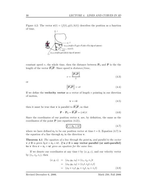
Figure 4.2: The vector r(t) = (f(t), g(t), h(t)) describes the position as a function
of time.
constant speed v, the whole time, then the distance between P 0 and P is the the
length of the vector −−→ P 0 P. Since speed is distance/time,
∥ −−→
P 0 P∥
v =
(4.3)
t
or
∥ −−→
P 0 P∥ = vt (4.4)
If we define the veclocity vector as a vector of length v pointing in our direction
of motion,
v = vˆv (4.5)
then it must be true that v is parallel to −−→ P 0 P, so that
P − P 0 = −−→ P 0 P = (vˆv) t (4.6)
Since the coordinates of our position vector r, are, by definition, the same as the
coordinates of the point P (see equation (4.2)),
r = r 0 + vt (4.7)
where we have defined r 0 to be our position vector at time t = 0. Equation (4.7) is
the equation of a line through r 0 in the direction v.
Theorem 4.1 The equation of a line through the point r 0 and parallel to the vector
v ≠ 0 is given by r = r 0 + vt. If u ≠ 0 is any vector parallel (or anti-parallel)
to v then r = r 0 + ut gives an equation for the same line.
If we denote our coordinates at any time t by (x, y, z), and our velocity vector
by (v x , v y , v z ), then
(x, y, z) = (x 0 , y 0 , z 0 ) + (v x , v y , v z )t
= (x 0 , y 0 , z 0 ) + (v x t, v y t, v z t)
= (x 0 + v x t, y 0 + v y t, z 0 + v z t) (4.8)
Revised December 6, 2006. Math 250, Fall 2006