Physics 403: Relativity Homework Assignment 4 Due 26 March ...

Physics 403: Relativity
Homework Assignment 4
Due 26 March 2007
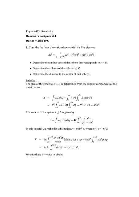
1. Consider the three dimensional space with the line element
ds 2 =
1
1 − r/R dr2 + r 2 (dθ 2 + sin 2 θ dφ 2 )
• Determine the surface area of the sphere that corresponds to r = R.
• Determine the volume of the sphere r ≤ R.
• Determine the distance to the center of that sphere.
Solution:
The area of the sphere at r = R is determined from the angular components of the
metric tensor:
A =
Z
ds θ ds φ =
Z π
= R 2 sinθ dθ
0
Z π
0
Z 2π
The volume of the sphere r ≤ R is given by
Z
V =
0
Z 2π
R dθ
0
Rsinθ dφ
dφ = R 2 · 2 · 2π = 4πR 2
Z R r 2 dr
ds r ds θ ds φ = 4π √
0 1 − r/R
In this integral we make the substitution r = Rsin 2 ρ, where 0 ≤ ρ ≤ π/2:
V
Z π/2 R 2 sin 4 Z
ρ
π/2
= 4π
0 cosρ 2Rsinρcosρ dρ = 8πR3 sin 5 ρ dρ
0
Z π/2
= 8πR 3 sinρ(1 − cos 2 ρ) 2 dρ
We substitute u = cosρ to obtain
0

Z 1
V = 8πR 3 du (1 − u 2 ) 2 = 8πR 3 8
15 = 64π
15 R3
0
This volume is somewhat larger than the volume of a sphere in Euclidean space,
4πR 3 /3.
The distance to the center of the sphere is again calculated from the metric tensor:
Z
D 0R = ds r =
Z R
0
Z √
dr
R R dr
[
√ = √ = −2 √ ] r=R
R(R − r) = 2R
1 − r/R 0 R − r r=0
Again, the distance s 0R is greater than the Euclidean distance, R.
2. The two dimensional torus can be embedded into three dimensional Euclidean
space by the relations
x
y
z
= Rcosθ [1+ρsinφ]
= Rsinθ [1+ρsinφ]
= Rρcosφ
where 0 < ρ < 1 is a fixed parameter. Compute the following quantities for the
torus, parametrized by (θ,φ):
• The metric tensor induced by the embedding from the Euclidean metric.
• The Christoffel symbols
• The Riemann curvature tensor.
• The Ricci scalar
Solution:
The infinitesimal Cartesian displacements (dx,dy,dz) are calculated in terms of
(dθ,dφ) as
dx
dy
dz
= −Rsinθ (1+ρsinφ) dθ+Rρcosθcosφ dφ
= Rcosθ (1+ρsinφ) dθ+Rρsinθcosφ dφ
= −Rρsinφ dφ

Thus we calculate the infinitesimal distance ds 2 :
ds 2 = dx 2 + dy 2 + dz 2 = R 2 (1+ρsinφ) 2 dθ 2 + R 2 ρ 2 dφ 2
The nonvanishing components of the metric tensor are g θθ = R 2 (1+ρsinφ) 2 and
g φφ = R 2 ρ 2 .
The Christoffel symbols are given by the formula
Γ λ µν = 1 2 gλρ [ ∂ ν g ρµ + ∂ µ g ρν − ∂ ρ g µν
]
The following Christoffel symbols are non-vanishing:
Γ φ cosφ (1+ρsinφ)
θθ
= −
ρ
Γ θ φθ = ρcosφ
Γθ θφ =
1+ρsinφ
The Riemann curvature tensor is
R α βγδ = ∂ γ Γ α βδ − ∂ δ Γ α βγ + Γα γε Γε βδ − Γα δε Γε βγ
The nonvanishing components of the Riemann tensor are
R φ θθφ
= −R φ θφθ = sinφ
ρ
(1+ρcosφ)
R θ φθφ = −R θ φφθ = ρsinφ
1+ρsinφ
The Ricci tensor is R µν = R λ µλν
. Its nonvanishing components are
The Ricci scalar curvature is
R θθ = sinφ
ρ
(1+ρsinφ)
ρsinφ
R φφ =
1+ρsinφ

R = g µν R µν = 2 sinφ
R 2 ρ 1+ρsinφ
We may compute the Killing vectors k µ = [k θ (θ,φ), k φ (θ,φ)] for this geometry by
solving the equations
That is,
∂ µ k ν + ∂ ν k µ − 2Γ λ µν k λ = 0
∂ θ k θ = Γ φ θθ k φ = − cosφ(1+ρsinφ)
ρ
∂ θ k φ + ∂ φ k θ = 2 Γ θ θφ k ρcosφ
θ = 2
1+ρsinφ k θ
∂ φ k φ = 0
From the last relation we conclude that k φ is independent of the variable φ. The
second relation can be written as
k φ
∂ φ k θ − 2
ρcosφ
1+ρsinφ k θ
[ ]
(1+ρsinφ) 2 k θ
∂ φ
(1+ρsinφ) 2
= −∂ θ k φ
= −∂ θ k φ
We define the quantity g(θ) = −∂ θ k φ , and write this equation as
( )
k θ
g(θ)
∂ φ
(1+ρsinφ) 2 =
(1+ρsinφ) 2
Let us integrate with respect to the variable φ to obtain
[
Z φ
k θ = (1+ρsinφ) 2 dφ ′ ]
f(θ)+g(θ)
π/2 (1+ρsinφ ′ ) 2
We insert this relation into the first Killing vector relation, to obtain
[
Z φ
(1+ρsinφ) 2 f ′ (θ)+g ′ dφ ′ ]
(θ)
π/2 (1+ρsinφ ′ ) 2 = − cosφ(1+ρsinφ) k φ
ρ

This equation must be satisfied at every value of the variable φ. Setting φ = π/2,
we establish that f ′ (θ) = 0 at all θ. Consequently,
Z φ
g ′ (θ)
π/2
dφ ′
(1+ρsinφ ′ ) 2 = − cosφ
ρ(1+ρsinφ) k φ(θ)
We differentiate both sides with respect to φ to obtain
g ′ [
]
(θ)
(1+ρsinφ) 2 = sinφ
ρ(1+ρsinφ) + cosφ
(1+ρsinφ) 2 k φ (θ)
Since the relation must also be true at all φ, it follows that k φ (θ) = 0 and g ′ (θ) = 0.
Furthermore, since g(θ) = −∂ θ k φ , it follows that g(θ) = 0. Consequently, f(θ) =
f 0 is a constant, and the only Killing vector is
k µ = f 0 [(1+ρsinθ) 2 ,0]
Note that the corresponding contravariant Killing vector is
k µ = g µλ k λ = f 0 [1,0]
The existence of this Killing vector may be established from the fact that the
metric tensor is independent of the coordinate θ. We have shown that it is the only
Killing vector for this metric geometry.
3. Show that for any two-dimensional manifold the covariant curvature tensor has
the form
R ab,cd = κ [g ac g bd − g ad g bc ]
where κ may be a function of the coordinates. Why does this result not generalize
to manifolds of higher dimensions?
Solution:
The covariant fourth order Riemann tensor has the following symmetry properties:
R ab,cd = −R ba,cd = −R ab,dc
In any two-dimensional space there can be only one independent component of
that tensor, since the indices (a,b) as well as (c,d), must be distinct.
Thus, of the 16 components of R ab,cd , we have

and all other components vanish.
The tensor
R 12,21 = −R 21,21 = −R 12,12 = R 21,12
g ac g bd − g ab g cd
has the same symmetry properties as R ab,cd , so that the two tensors must be proportional:
R ab,cd = κ [g ac g bd − g ab g cd ]
where κ may depend upon the two coordinates (u 1 ,u 2 ).
For the example considered in Problem 2, we have
R φθ,θφ
= g φφ R φ θθφ = −R2 ρsinφ (1+ρsinφ)
R θφ,θφ
= g θθ R θ φθφ = R2 ρsinφ (1+ρsinφ)
g θθ g φφ = R 4 ρ 2 (1+ρsinφ) 2
The structure is evident in this case, with
κ =
Note that the scalar curvature is R = 2κ.
sinφ
ρR 2 (1+ρsinφ)
4. Consider the Hyperbolic Plane defined by the metric
ds 2 = dx2 + dy 2
y 2
where y ≥ 0. Show that the geodesics are semi-circles centered on the x-axis or
vertical lines parallel to the y-axis. Determine x(s) and y(s) as functions of the
length s along these curves.
Solution:
The line element ds 2 is invariant under a change in the scale of coordinates;
(x,y) → (λ x,λ y). The components of the metric tensor are

g xx = 1/g xx = 1/y 2
g yy = 1/g yy = 1/y 2
g xy = g yx = 0
The Christoffel symbols are determined by the formula
Γ λ µν = 1 2 gλρ[ ]
∂ ν g ρµ + ∂ µ g ρν − ∂ ρ g µν
The non-vanishing Christoffel symbols are
Γ x xy = Γ x yx
= 1 2 gxx ∂ y g xx = − 1 y
Γ y xx
= − 1 2 gyy ∂ y g xx = 1 y
Γ y yy
= 1 2 gyy ∂ y g yy = − 1 y
The Riemann tensor may be computed from the Christoffel symbols:
R x yxy = −∂ y Γ x yx + Γx xy Γy yy − Γx yx Γx xy = − 1 y 2
R xyxy = g xx R x yxy = − 1 y 4
All other components of the Riemann tensor may be obtained using the formula
in Problem 3, with κ = −1. Note that the scalar curvature is R = −2, and that it is
scale-invariant.
The equation for the geodesics u α (s) is
That is,
d 2 u α
ds 2
d 2 y
ds 2 + 1 y
+ Γα βγ
du β
ds
du γ
ds = 0
d 2 x
ds 2 − 2 dx dy
= 0
y ds ds
( dx 2
−
ds) 1 ( ) dy 2
= 0
y ds

It follows from the definition of the metric
that
ds 2 = dx2 + dy 2
y 2
( ) dx 2 ( ) dy 2
+ = y 2
ds ds
(This relation may also be obtained from the geodesic equations themselves.) We
use this relation to case the geodesic equation for y(s) into the form
( )
y d2 y dy 2
ds 2 + y2 = 2
ds
Adopting the notation y ′ = dy/ds, we may write
d 2 y
ds 2 = dy′
ds = dy′
dy
Thus the geodesic equation for y takes the form
dy dy′
= y′
ds dy
y y ′ dy′
dy + y2 = 2y ′2
This is a nonlinear first order differential equation for y ′ as a function of y; y ′ (y).
We express it in terms of t(y) = y ′2 :
or
y
2
dt
dy + y2 = 2t
dt
dy − 4 y t = −2y
We multiply this linear first order differential equation for t by the integrating
factor 1/y 4 and solve it:

1 dt
y 4 dy − 4 y 5 t = − 2 y
( )
3
d t
dy y 4 = d ( ) 1
dy y 2
t
y 4 = −κ 2 + 1 y 2
t = y 2 − κ 2 y 4
Equivalently, we have
y ′ = dy
ds
dy
y 2√ 1/y 2 − κ 2
= y √ 1 − κ 2 y 2
= ds
Let us define the variable u(s) = 1/y(s), so that du = −dy/y 2 and
du
√
u 2 − κ 2 = −ds
This equation may be integrated directly to obtain u = κcosh(s − s 0 ), or
y(s) =
1
κcosh(s − s 0 )
We may calculate x(s) using this result for y(s) the metric tensor relation:
( ) dx 2 ( ) dy 2
= y 2 − = y 2 − y 2 (1 − κ 2 y 2 ) = κ 2 y 4
ds
ds
We take the positive square root to have
Consequently,
dx
ds = κ = 1
κcosh 2 (s − s 0 )
x − x 0 = 1 κ tanh(s − s 0)

We also obtain
(x − x 0 ) 2 + y 2 = 1+sinh2 (s − s 0 )
κ 2 cosh 2 (s − s 0 ) = 1 κ 2
The geodesic trajectory is thus a circle of radius R = 1/κ centered at the point
(x 0 ,0), which lies on the x-axis. Actually, because y(s) is always positive, we
should regard it as a semi-circle in the upper half y-plane. In the limiting case
κ → 0, the geodesics become half-lines, x = x 0 ; y > 0.
To summarize, the geodesic trajectory is parametrized by the formulas
y(s) =
R
cosh(s − s 0 )
x(s) = x 0 + R sinh(s − s 0)
cosh(s − s 0 )
Actually, we can solve for the trajectory y(x) more directly by determining the
paths of minimum length
Z Z √
x2
1+y ′ 2
S = ds =
dx
x 1 y
Because the “effective Lagrangian”
L =
√
1+y ′ 2
does not involve the dependent variable x, the “Jacobi integral” is a constant of
the motion:
y
y ′ ∂L
∂y ′ − L
√
y ′ 2 1+y ′
y √ 1+y − 2
′ 2 y
1
√
y √ 1+y ′ 2
= J = − 1 R
= − 1 R
= 1 R
1+y ′2 = R y
√
y ′ R
=
2
y 2 − 1

We integrate this equation to obtain
Z y
y dy
√ =
R 2 − y 2
Z x
dx = x − x0
− √ R 2 − y 2 = x − x 0
(x − x 0 ) 2 + y 2 = R 2
To determine the arc length of a path, we use the original metric formula:
ds
dx
=
ds =
√
1+y ′ 2
= R y y 2 = R
R 2 −(x − x 0 ) 2
Rdx
R 2 −(x − x 0 ) 2
We make the substitution x = x 0 + R sinθ to obtain
ds = R secθ dθ
s − s 0 = ln(secθ+tanθ)
e s−s 0
= secθ+tanθ
sec 2 θ = tan 2 θ − 2 tanθ e s−s 0
+ e 2(s−s 0)
tanθ = sinh(s − s 0 )
Note also that sinθ = tanh(s − s 0 ), so that
x − x 0 = R tanh(s − s 0 )
R
y = R cosθ =
cosh(s − s 0 )
5. In a four-dimensional Minkowski space with coordinates (t,x,y,z), a 3-hyperboloid
is defined by t 2 − x 2 − y 2 − z 2 = R 2 . Show that the metric on the 3-surface of the
hyperboloid can be written in the form
−ds 2 = R 2 [dχ 2 + sinh 2 χ (dθ 2 + sin 2 θ dφ 2 ) ]

Show that the total volume of the 3-hyperboloid is infinite.
Solution:
Let us define the coordinates (χ,θ,φ) in terms of (t,x,y,z) by
t
z
y
x
= Rcoshχ
= Rsinhχ cosθ
= Rsinhχ sinθ sinφ
= Rsinhχ sinθ cosφ
With these coordinates, we automatically impose the constraint t 2 −x 2 −y 2 −z 2 =
R 2 . The corresponding changes in these coordinates are
dt
dz
dy
dx
= Rsinhχ dχ
= Rcoshχcosθ dχ − Rsinhχsinθ dθ
= Rcoshχsinθcosφ dχ+Rsinhχcosθsinφ dθ − Rsinhχsinθcosφ dφ
= Rcoshχsinθcosφ dχ+Rsinhχcosθcosφ dθ − Rsinhχsinθsinφ dφ
The Minkowski space metric may thus be written
ds 2
= dt 2 − dz 2 − dy 2 − dz 2 = −ds 2 χ − ds 2 θ − ds2 φ
= −R 2 dχ 2 − R 2 sinh 2 χ dθ 2 − R 2 sinh 2 χsin 2 θ dφ 2
The total three-volume of the hyperboloidal region χ ≤ χ 0 is
Z
Z χ0
Z π
Z 2π
V = ds χ ds θ ds φ = R dχ Rsinhχ dθ Rsinhχsinθ dφ
0 0
0
Z χ0
Z χ0
= 4πR 3 sinh 2 χ dχ = 2πR 3 (cosh2χ − 1) = πR 3 (sinh2χ 0 − 2χ 0 )
0
0
The volume becomes infinite in the limit χ 0 → ∞.
We could determine the geodesics for this surface by obtaining and solving the
geodesic equations for (χ(s),θ(s),φ(s)). Instead, we will analyze the geodesic
equations for (t(s),x(s),y(s),z(s)), using Lagrange multipliers to impose the constraint

The modified Lagrangian is
[ ( ) dt 2
L = −
ds
t(s) 2 − x(s) 2 − y(s) 2 − z(s) 2 = R 2
( ) dx 2
−
ds
The Euler-Lagrange equations are
( ) dy 2
−
ds
( ) ]
dz
2
+ κ 2[ t 2 − x 2 − y 2 − z 2]
ds
d 2 t
ds 2 − κ2 t = 0
d 2 x
ds 2 − κ2 x = 0
d 2 y
ds 2 − κ2 y = 0
d 2 z
ds 2 − κ2 z = 0
The solution that passes through the first point on the hyperboloid, (t 1 ,x 1 ,y 1 ,z 1 )
at s = 0, is
t(s) = t 1 coshκs+d sinhκs
x(s) = x 1 coshκs+asinhκs
y(s) = y 1 coshκs+bsinhκs
z(s) = z 1 coshκs+csinhκs
We the curve satisfies the constraint
t(s) 2 − x(s) 2 − y(s) 2 − z(s) 2 = R 2
under the following conditions:
t 2 1 − x2 1 − y2 1 − z2 1 = R 2
t 1 d − x 1 a − y 1 b − z 1 c = 0
a 2 − b 2 + c 2 − d 2 = R 2

The parameter κ can be determined from the constraint
( ) dt 2
−
ds
At s = 0 we obtain the relation
( ) dx 2
−
ds
( ) dy 2
−
ds
κ 2 (d 2 − a 2 − b 2 − c 2 ) = −1
( ) dz 2
= −1
ds
or κR = 1. Under the conditions given above, this relation is satisfied everywhere
on the curve.
Next we determine S, the path length on the hyperboloid between the points
(t 1 ,x 1 ,y 1 ,z 1 ) and (t 2 ,x 2 ,y 2 ,z 2 ):
t 2 −t 1 coshρ
x 2 − x 1 coshρ
y 2 − y 1 coshρ
z 2 − z 1 coshρ
= d sinhρ
= asinhρ
= bsinhρ
= csinhρ
where ρ = κS = S/R. We square these terms and combine them to determine the
parameter ρ:
(t 2 −t 1 coshρ) 2 −(x 2 − x 1 coshρ) 2 −(y 2 − y 1 coshρ) 2 −(z 2 − z 1 coshρ) 2
= (d sinhρ) 2 −(asinhρ) 2 −(bsinhρ) 2 −(csinhρ) 2 ;
R 2 − 2(t 1 t 2 − x 1 x 2 − y 1 y 2 − z 1 z 2 )coshρ+R 2 cosh 2 ρ = −R 2 sinh 2 ρ ;
(t 1 t 2 − x 1 x 2 − y 1 y 2 − z 1 z 2 )coshρ = R 2 cosh 2 ρ ;
coshρ = (t 1 t 2 − x 1 x 2 − y 1 y 2 − z 1 z 2 )/R 2 .
One may show that t 1 t 2 − x 1 x 2 − y 1 y 2 − z 1 z 2 ≥ R 2 , so that coshρ ≥ 1.
t 1 t 2 − x 1 x 2 − y 1 y 2 − z 1 z 2 =
≥
√ √r1 2 + R2 r2 2 + R2 −⃗r 1 ·⃗r 2
√ √r1 2 + R2 r2 2 + R2 − r 1 r 2
Furthermore, we have

(r 1 − r 2 ) 2 ≥ 0 ;
(r 2 1 + R 2 ) (r 2 2 + R 2 ) ≥ (r 1 r 2 + R 2 ) 2 ;
√r 2 1 + R2 √
r 2 2 + R2 ≥ r 1 r 2 + r 2 .
The result is established. The coefficients (a,b,c,d) can then be determined:
d
a
b
c
= (t 2 −t 1 coshρ)/sinhρ
= (x 2 − x 1 coshρ)/sinhρ
= (y 2 − y 1 coshρ)/sinhρ
= (z 2 − z 1 coshρ)/sinhρ
They automatically satisfy the relation a 2 + b 2 + c 2 − d 2 = R 2 . In addition, we
may show by direct substitution that
t 1 d − x 1 a − y 1 b − z 1 c = 1
sinhρ [(t 1t 2 − x 1 x 2 − y 1 y 2 − z 1 z 2 ) − R 2 coshρ] = 0
as required. The geodesic curve on the hyperboloid lies on a plane passing through
the origin:
α x(s)+β y(s)+γ z(s)+δ t(s) = 0
The parameters (α,β,γ,δ) must satisfy the constraints
α x 1 + β y 1 + γ z 1 + δ t 1 = 0
α x 2 + β y 2 + γ z 2 + δ t 2 = 0
The solution for (α,β,γ,δ) is not unique. In fact, there is a two-parameter family
of such planes in four-dimensional Minkowski space.
This hyperboloid is a three dimensional surface in four-dimensional Minkowski
space. the (Euclidean) length on this surface is
so that
−ds 2 = R 2 [dχ 2 + sinh 2 χ (dθ 2 + sin 2 θ dφ 2 ) ]

g χ χ = R 2
g θ θ
g φ φ
= R 2 sinh 2 χ
= R 2 sinh 2 χ sin 2 θ
The following Christoffel symbols are non-vanishing:
Γ χ θ θ
Γ χ φ φ
Γ θ θ χ = Γθ χ θ
= 1 2 gχ χ (−∂ χ g θ θ ) = −sinhχ coshχ
= 1 2 gχ χ (−∂ χ g φ φ ) = −sinhχ coshχ sin 2 θ
= 1 2 gθ θ (∂ χ g θ θ ) = coshχ
sinhχ
Γ θ φ φ
= 1 2 gθ θ (−∂ θ g φ φ ) = −sinθ cosθ
Γ φ φ χ = Γφ χ φ
= 1 2 gφ φ (∂ χ g φ φ ) = coshχ
sinhχ
Γ φ φ θ = Γφ θ φ
= 1 2 gφ φ (∂ θ g φ φ ) = cosθ
sinθ
The non-vanishing components of R a bcd
(along with their antisymmetric counterparts
R a bdc = −Ra bcd ) are
R χ θ χ θ
R χ φ χ φ
R θ χ θ χ
R θ φ θ φ
R φ χ φ χ
R φ θ φ θ
= ∂ χ Γ χ θ θ − Γχ θ θ Γθ θ χ = −sinh2 χ
= ∂ χ Γ χ φ φ − Γχ φ φ Γφ φ χ = −sinh2 χsin 2 θ
= ∂ χ Γ θ χ θ − Γθ χ θ Γθ χ θ = −1
= ∂ θ Γ θ φ φ + Γθ θ χ Γχ φ φ − Γθ φ φ Γφ θ φ = −sinh2 θ sin 2 φ
= −∂ χ Γ θ χ θ − Γθ χ θ Γθ θ χ = −1
= −∂ θ Γ φ θ φ+Γ φ φ χ Γχ θ θ − Γφ θ φ Γφ θ φ = −sinh2 χ
The diagonal components of the Ricci tensor are
R χ χ
R θ θ
R φ φ
= −2
= −2sinh 2 χ
= −2sinh 2 χ sin 2 θ

The Ricci scalar is given by the simple formula R = −2.