PROOF COVER SHEET

PROOF COVER SHEET 

Journal acronym: TGIS 

Author(s): Shiuan Wan, Tsu-Chiang Lei and Tein-Yin Chou 

Article title: A landslide expert system: image classification through integration of 

data mining approaches for multi-category analysis 

Article no: 613397 

Enclosures: 1) Query sheet 

2) Article proofs 

Dear Author, 

1. Please check these proofs carefully. It is the responsibility of the corresponding 

author to check these and approve or amend them. A second proof is not normally 

provided. Taylor & Francis cannot be held responsible for uncorrected errors, even if 

introduced during the production process. Once your corrections have been added to the 

article, it will be considered ready for publication. 

For detailed guidance on how to check your proofs, please see 

http://journalauthors.tandf.co.uk/production/checkingproofs.asp. 

2. Please review the table of contributors below and confirm that the first and last 

names are structured correctly and that the authors are listed in the correct order of 

contribution. This check is to ensure that your name will appear correctly online and 

when the article is indexed. 

Sequence Prefix Given name(s) Surname Suffix 

1 Shiuan Wan 

2 Tsu-Chiang Lei 

3 Tein-Yin Chou

Queries are marked in the margins of the proofs. Unless advised otherwise, submit all 

corrections and answers to the queries using the CATS online correction form, and then 

press the “Submit All Corrections” button. 

AUTHOR QUERIES 

General query: You have warranted that you have secured the necessary written 

permission from the appropriate copyright owner for the reproduction of any text, 

illustration, or other material in your article. (Please see 

http://journalauthors.tandf.co.uk/preparation/permission.asp.) Please check that any 

required acknowledgements have been included to reflect this. 

AQ1 

AQ2 

AQ3 

AQ4 

AQ5 

AQ6 

AQ7 

AQ8 

AQ9 

AQ10 

AQ11 

AQ12 

AQ13 

Please provide the department name for the author “Chou”, if applicable. 

Please provide the expansion for SPOT, if applicable. 

Please check whether the year is correct as inserted for the author “Wan” in 

the sentence “Wan (2009) used a ...”. 

Please check whether the edits to the sentence “In the past, in this ...”are 

correct. 

The citation ’Lee and Vachtsevanos, 2002’ has not been included in the 

reference list. Please check. 

The sense of the sentence “Then, the modification of Thematic Map ...”is 

not clear. Please consider rephrasing for clarity. 

The citation ‘Wan and Yen 2006’ has not been included in the reference list. 

Please check. 

Please check whether any term is missing after the phrase “given in” in the 

sentence “The method for extracting ...”. 

Please provide the expansion for ERDAS, if applicable. 

The sense of the sentence “Different atmospheric condition can result in 

different qualities of Figure” is not clear. Please check. 

The reference citation “Sinha and Laplante 2004” not included in the 

reference list. Please provide. 

Both the terms “k-means” and “K-means” are present in the text. As such, the 

term “k-means” has been changed to “K-means” throughout. Please check 

whether this is OK. 

Please check whether the temporary citation of Table 6 is correct as inserted 

here. 

AQ14 As there are three authors, the acknowledgement section has been changed 

accordingly. Please check whether this is OK. 

AQ15 Please provide the citation for the reference “Baeza and Corominas, 2001”.

AQ16 Please provide the place and date of the proceedings, publisher name and 

location, and editor group for the reference “Deogun et al. 1994”, if 

applicable. 

AQ17 Please provide the place and date of the proceedings, publisher details and 

editor group for the reference “Katzberg and Ziarko 1993”, if applicable. 

AQ18 Please provide the access date for the reference “Lee and Choi 2004a”. 

AQ19 Please provide the access date for the reference “Lin 2008”. 

AQ20 Please provide the access date for the reference “Lin et al. 2007”. 

AQ21 Please provide the citation for the reference “Maleta et al. 2005”. 

AQ22 Please provide the publisher name and location and the date of the proceeding 

for the reference “Nguyen and Skowron 1995”. 

AQ23 Please provide the publisher name and location for the reference “Nguyen and 

Nguyen 1998b”. 

AQ24 Plesae provide the access date for the reference “RSES 2.2 User’s Guide, 

2005”. 

AQ25 Table 3a and b has been set as Tables 3 and 4, respectively, and the subsequent 

tables renumbered. Please check whether this is OK.

International Journal of Geographical Information Science 

Vol. 00, No. 00, Xxxx 2011, 1–24 

A landslide expert system: image classification through integration of 

data mining approaches for multi-category analysis 

Shiuan Wan a *, Tsu-Chiang Lei b and Tein-Yin Chou c 

AQ1 

a Department of Information Management, Ling Tung University, Taichung, Taiwan; b Department of 

Urban Planning and Spatial Information, Feng Chung University, Taichung, Taiwan; c GIS Center, 

Feng Chia University, Taichung, Taiwan 

(Received 16 February 2011; final version received 4 August 2011) 

5 

Remote Sensing (RS) data can assist in the classification of landscapes to identify 

landslides. Recognizing the relationship between landform/landscape and landslide 

areas is, however, complex. Soil properties, geomorphological, and groundwater condi- 10 

tions govern the instability of slopes. Previous study of Wan (2009; A spatial decision 

support system for extracting the core factors and thresholds for landslide susceptibility 

map. Engineering Geology, 108, 237–251) used the maximum-likelihood classifier to 

classify the multi-category landslide image data. Unfortunately, the classification does 

not consider the geomorphologic condition. Accordingly, a Landslide Expert System 15 

was developed to modify these problems. The system uses multi-date SPOT image data 

to develop the landslide database. The threshold slope which becomes vulnerable to 

landslides is obtained by the K-means method. Then, an innovative Data Mining technique 

– Discrete Rough Sets (DRS) – is applied to obtain the core variables and their 

relevant thresholds. Finally, the Expert Knowledge Translation Platform (EKTP) is used 20 

to create the rules for classification. This study used a new approach called ‘Rough Set 

Tree’ to demonstrate the performance of the approach. The classification of landslide 

vulnerable areas, bare land, rock, streams, and water-body is greatly improved. 

Keywords: expert system; landslide; data mining 

AQ2 

1. Introduction 25 

In general, landslides are dramatic events in the progressive degradation of a slope. They 

are usually driven by rainfall or gravity forces, but may be triggered by tectonic movement 

(Mayoraz et al. 1996, Floris et al. 2004). The tendency of a slope to move is described 

as the instability of the slope, whereas the failures are described as the actual mass movement. 

This may occur along well-defined planes with large catastrophic displacements or 30 

by slow movement. Although slopes are likely to degrade over time, movement still may 

be triggered into more dramatic failure by a variety of natural or manmade activities. That 

is, a landslide occurs when the shear stresses within the slope exceed the shear strength 

of the soil. Therefore, geomorphologic investigations become crucial to yield information 

about the stability of topographic features in a particular study area. Vegetation can 35 

greatly influence the surface runoff and reduce the pore water pressure and water content 

of the soil (Huete 1988). Simple numerical vegetation indices can be used to describe 

*Corresponding author. Email: shiuan123@mail.ltu.edu.tw 

ISSN 1365-8816 print/ISSN 1362-3087 online 

© 2011 Taylor & Francis 

DOI: 10.1080/13658816.2011.613397 

http://www.informaworld.com

2 S. Wan et al. 

the vegetation condition on a slope. In this study, vegetation conditions and slope are two 

important variables for generating a landslide susceptibility map. 

To observe the vegetation condition and slope instability, satellite Remote Sensing (RS) 40 

images and Digital Elevation Model (DEM) data are used. The capability of RS image data 

to provide information about vegetation conditions over extensive areas is well accepted 

(Lin et al. 2006). DEMs are widely used to study the morphological characteristics of the 

landform (Lin et al. 2007, Lin 2008). 

Although the DEM and RS data are important for mapping landslide, an efficient deci- 45 

sion system is necessary to model the simulated occurrence of a landslide. Unfortunately, 

few decision systems integrate RS and DEM data. Landslide hazard mapping is often 

performed by intersecting hillslope instability factors and vegetation conditions, with the 

result usually managed as a Thematic Map (Bannari et al. 1995, Mayoraz et al. 1996). 

There are two kinds of decision systems: (1) a decision support system (DSS) and (2) an 50 

expert system (DS). Decision systems are now widely applied in many fields. 

A fundamental question arises: how to develop these decision systems efficiently? For 

instance, an effective DSS for landslide risk (Wan 2009) usually requires (1) an integration 

system to collect the environmental data (by either RS or DEM); (2) a data-driven 

method to search for the best representative study dataset (such as cross validation method); 55 

and (3) a good classifier. In his study, Wan (2009) used a maximum-likelihood classifier 

(MLC). The classification accuracy was about 77.8% but improvements were needed to 

discriminate between different categories. However, resolving the difficulties of the classification 

of various categories involves a great deal of expert knowledge (Ziarko 1991, 

Zerger 2002, Wan et al. 2009, Pradhan and Lee 2010, Wan et al. 2010a). The objective of 60 

this study is to develop an ES to enhance the accuracy. The resolution consisted of correcting 

the following issues: (1) A threshold of slope is found to distinguish many of the 

‘easily confused’ categories, such as bare land and channels. For instance, rock, streams, 

and landslide are easily confused categories in image classification. (2) A translation 

scheme is generated to transfer the incorrectly classified samples into correct categories. 65 

This experience was of help in constructing an ES to enhance the accuracy of prediction 

effectively. 

To sum up, enhancing the prediction accuracy of the classification of landslide risk 

involves (1) the selection of a classifier and (2) a translation platform created from expert 

knowledge. The categories discriminated by classifier in this study include water-body, 70 

stream, grassland, timberland, landslide area, bare land (rock), and potential landslide area 

(sensitivity area). In the past, in this sort of classification application, statistical models 

from a set of given data were generally used. In typical studies, a learning algorithm passively 

accepts randomly selected training examples. Providing labeled examples is costly 

in terms of human time and effort (Lee and Choi 2004). Selected training examples of 75 

this type may be quite biased. For example, some researchers describe a Support Vector 

Machine (SVM) for the prediction of landslides or debris flows (Yesilnacar and Topal 

2005, Wan and Lei 2009, Yilmaz 2009) which was trained by a few selected training 

examples. The classification outcomes were found to remain the same if all data except 

the support vectors were omitted from the training set. Thus, only a few examples define 80 

the separating surface and all the rest were redundant to the classifier. Given that experience, 

we planned to develop an ES which integrates a Data Mining approach with 

an effective translation strategy. Specifically, the complexity of landform categories versus 

the landslide occurrence is a difficult problem; therefore, we developed an Expert 

Knowledge Translation Platform (EKTP) to tackle the performance of landslide occurrence 85 

classification. A similar concept is presented in Ahlqvist (2005). 

AQ3 

AQ4

International Journal of Geographical Information Science 3 

In recent years, Data Mining in the geosciences (Lei et al. 2008, Wan et al. 2010b) has 

identified new approaches. Also, the development of DSS and ES provides pathways to 

integrate different sources of data to enhance the quality of classification. The main problems 

that can be approached using Rough Set theory include rough classification (Deogun 90 

et al. 1994, Słowiński et al. 1994), reduction of an information system (Katzberg and 

Ziarko 1993), discovery of data dependencies (Ziarko 1991, Ahlqvist et al. 2000, 2003), 

and other new Data Mining applications (Deogun et al. 1994). Accordingly, we consider 

Rough Set theory (Pawlak 1982, 1991) as the engine of DSS or ES to handle the vagueness 

and uncertainty of data (Pawlak et al. 1995, Lee and Vachtsevanos 2002). 

95 

The advantage of Discrete Rough Set (DRS) over Rough Set is that it can handle continuous 

data and transform them into a discrete dataset (Nguyen and Skowron 1995, Nguyen 

and Nguyen 1998a, 1998b). Not much work has been done in the feature selection field of 

image classification using this technique (Leung et al. 2007). Such research can offer three 

crucial advantages: 100 

AQ5 

(1) Dimensional reduction: dimension reduction is the process of reducing the number 

of random variables under consideration (Kirshnaiash and Kanal 1982). 

(2) Thresholds: the image classification from the cutting points of core attributes. 

(3) DRS provides ancillary criterion rules for each of the attributes obtained from the 

image datasets. 105 

As mentioned above, this is completely different from the traditional deterministic or statistical 

methods that require predetermined ‘weights’(Van Westen et al. 2003, Lee et al. 

2004) and assume distributions (such as uniform distribution or normal distributions) in 

the independent variables. Taking advantage of the benefits of the DRS, therefore, our 

study integrated the DRS to display the following process: 110 

(1) We study the soil properties, slope instability, and vegetation conditions. We 

initially use K-means to find the threshold of slope instability from the DEM 

data. Then, we use the DRS to generate significant image features of vegetation 

conditions by original RS image data with ancillary vegetation indicators. 

(2) We also discover the image classification tree-rules through DRS, providing crucial 115 

information for decision making. 

(3) Based on the observations on the changes of categories (such as water-body, 

timberland, sensitive area, rock, stream, and landslide) before/after a landslide, 

we develop an ancillary tool EKTP to improve the efficiency of multi-category 

classification. 120 

A review of the literature suggests that it is important to test the Rough Set tree as a tool to 

enhance the classification efforts (Ananthanarayana et al. 2003, Wei et al. 2005). Hence, 

our research has two parts: (1) A series of DEM data are used to find the threshold of 

slope for landslide occurrence. (2) The DRS method is applied to tackle the RS data. 

Another important contribution of this study is to generate a Rough Set tree to describe 125 

the occurrence of a landslide in our study area. In the process of constructing a tree, the 

criteria of selecting test attributes will influence the classification accuracy of the tree. In 

this study, the degree of dependency of condition attributes (input variables) to decision 

attributes (output decisions) is found. DRS theory is used as a heuristic way to select the 

attribute that will accurately separate the samples into individual classes (Pawlak 1982, 130 

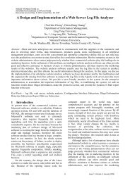
1991, Pawlak et al. 1995, Walaczak and Massart 1999, Goh and Law 2003). Figure 1


Discrete rough set 

Seven bands of 

RS image 

Sampling 

Thresholds of slope 

Accuracy 

rate 

Theme map 

Arc-Gis 

program 

Core factor 

with thresholds 

Knowledge 

database 

Figure 1. 

The steps for Discrete Rough Set + Theme Map. 

shows the steps of the DRS and how the Thematic Map is generated. We used three original 

image bands and four ancillary information as the study material. Then, we selected 

45 samples of image data to study the relations between the landslide occurrences versus 

nonoccurrences. The classifier DRS (developed by Rough Set Exploration System 135 

(RSES)) is used to attain the core factors and thresholds (through dimensional reduction). 

Then, the spatial knowledge database is generated. Next, we study the samples and use 

the thresholds of the selecting samples to create EKTP by the slopes. The first classification 

process was done by DRS and then the Thematic Map is created initially. Then, 

the modification of Thematic Map enhances the performance accuracy was based on the 140 

EKTP. Finally, the multi-category classification was presented by Rough Set-based tree 

structure. 

AQ6 

2. Study area, scenario, and materials 

2.1. Study area 

In general, the analyses of landslide occurrences usually rely on inventory maps. 145 

Unfortunately, the study area is short of historical data of landslides and the inventory 

map does not exist. In this research, the study area is selected at Shei-Pa National Park 

(see Figure 2a) and the data collected belong to the period after the Chi-Chi earthquake. 

Accordingly, a good case study of fracture geology may contain complicated geology 

and fault crossover. The entire area is surrounded by giant woods with natural beautiful 150 

scenery. The study area in the central part of Taiwan (E 121:13:39, N 24:09:57). The Shei- 

Pa National Park (area: 75,000 ha.) is situated 40–80 km from the Chelung Pu fault, which 

transmitted tremendous energy to the central part of Taiwan during this event. Utilizing 

DEMs, SPOT-image data, field investigation, and the attribute data from GIS (morphology, 

geology, landslide, slope, soil type, and so on), we built a new database for observing 155 

landslide events. 

To derive the geomorphological data, we relied on a well-developed DEM database. 

This was used to construct a series of knowledge rules for landslide occurrence. The 

DEM was a subset clipped from the DEM database of Taiwan by the Center for Space


Figure 2. The (a) location, (b) 2006/07/29, (c) 2006/10/20 remote sensing images, and 

(d) 3D-DEM model image data. 

and Remote Sensing Research, National Central University. The DEM database of Taiwan 160 

had a resolution of 40 m × 40 m. This study made use of two different SPOT image scenes 

(2006/7/29 and 2006/10/20). The size of each pixel is 20 × 20 (m) resampled to match 

the resolution of the DEM data.


2.2. Scenario 

In our study, a catastrophic earthquake occurred on 21 September 1999 in Central Taiwan. 165 

The seismic magnitude reached 7.3 on the Richter scale at the center. The Chi-Chi earthquake 

triggered many landslides, dammed lakes and a large number of people were killed. 

The damage caused by this earthquake was the result of numerous issues including urban 

and rural development, land utilization, and soil and water conservation. Usually, the average 

rainfall is about 3000–4200 mm/year. Two years later, typhoon Toraji brought a heavy 170 

rainfall (about 1750 mm in 3 days) causing more landslides. A large number of these landslides 

have been mapped from SPOT images and some of these are verified by a detailed 

field investigation. Figure 2b and c presents the two different scenarios of the monitoring 

time. The key point of using these images is to observe the changes for landscape which 

will be a good resource for landslide analysis. 175 

2.3. Spatial database and expert’s experiences 

The environmental landslide database included two indicators: (1) slope and the elevation 

and (2) the spectrum of image data and vegetation indicators. In the first part, the slope 

data are calculated from DEM data. Applying the DEM data, the elevations of observation 

spots were attained. Then, the slopes of those spots are calculated: (1) the average elevation 180 

is about 1200–1800 m and (2) the average slope is 23.78 ◦ with standard deviation of 4.7 ◦ . 

The instability of the slope is usually governed by soil type and the slope of the landforms 

(Wan et al. 2008). Figure 2d shows one of the profiles of 3D-DEM model of the Shei-Pa 

National Park. The vegetation indices were derived from our SPOT image dataset. 

2.4. Type of landslide 185 

The landslides triggered by the Chi-Chi earthquake can be classified into four broad categories: 

(1) ubiquitous, relatively shallow slides on very steep slopes underlain by stiff soils 

and jointed rock; (2) rock falls; (3) sparse deep seated failures; and (4) rare, very large 

coherent deep seated landslides (Khazai and Sitar 2003). In our study, the initial material 

for analysis of landslide samples included geology data, soil distribution map, and eleva- 190 

tion map. The soil type and soil depth were measured and then the engineering analysis 

of stability taken into account for the factors of slope and elevation (see next section). 

However, slopes with different soil-type conditions (such as permeability) behave differently 

in response to rainfall process or earthquake excitations (Khazai and Sitar 2003, Hong 

et al. 2005). In this research, the assumption of study area with regard to slope failures is 195 

similar (see Wan et al. 2010b for the detailed process of categorizing the soil type). Thus, 

it is presumed the soil type and soil depth are similar for each analyzed sample. Hence, 

their stability problems of slope failures are analyzed rationally. 

3. Research methods 

3.1. Applying K-means to search the threshold of slope instability 200 

K-means is an iterative clustering algorithm where items (or samples) are moved among 

sets of clusters until the desired sets are reached (Wan and Yen 2006). The cluster center 

is defined as the mean value of each cluster. While implementing K-means, the first step is 

to assign number of clusters and the initial value for each cluster center. Then, assign each 

items (or samples) to the cluster, which has the closest center, and to calculate the new 205 

AQ7


mean value for each cluster as a new center. Repeat this step until the convergence criteria 

are met. The algorithm is inherently iterative. The performance of the K-means depends 

on the initial positions of the cluster center, thereby making it advisable either to employ 

proper initial cluster or to allow more iterations (Rand 1971, Darken, and Moody 1990). 

3.2. Prominent classifier-DRS method 210 

This study focuses on a new technique of Data Mining scheme – Rough Set. The difference 

between conventional Rough Set and DRS is that data in conventional Rough Set must be 

predetermined in different groups/classes and DRS can handle continuous data and transform 

them into a discrete dataset. Furthermore, the DRS provides classification rules from 

the image data. This renders the knowledge database efficient for maximum separation 215 

among the categories in image classification. 

3.2.1. Rough Sets theory and discretization process (Nguyen and Skowron 1995) 

There are three stages involved in DRS. In the first stage, the ‘Information Table’ must 

be developed for the description of the characteristic attributes (inputs). In this table, a 

relation in a multi-attribute set is displayed. Then, all the attributes must be clustered into 220 

appropriate classes to construct a ‘Decision Attribute.’ The final step is to obtain the Cores 

and Reducts of the data attributes. Reducts and Cores are two fundamental concepts related 

to attribute reduction. The minimal subsets of attributes that discriminate equivalent classes 

of the relation, which is discriminable by the entire set of attributes, are called Reducts. The 

Core is the common part of all Reducts. 225 

3.2.1.1. RS theory to discretization the attribute values. The RS theory, first described by 

Pawlak (1982), is a formal approximation of a crisp set (i.e., conventional set) in terms of 

a pair of sets which give the lower and upper approximation of the original set. 

Step 1: Create information system table (I) 

Let I = (U, A) be an information system (attribute-value system), where U is a nonempty 230 

set of finite objects (the universe) and A is a nonempty, finite set of attributes such that 

a : U → V a for every a ∈ A. V a is the set of values that attribute a may take. With any 

P ⊆ A, there is an associated equivalence relation IND(P): 

IND(P) = { (x, y) ∈ U 2∣ ∣ ∀a ∈ P, a(x) = a(y) 

} 

(1) 

The partition of U generated by IND(P) is denoted U/IND(P) and can be calculated as 

follows: 235 

U/IND(P) =⊗{U/IND({a})| a ∈ P} (2) 

where U is the universe of the dataset; the symbol of ‘/’ is to cut the U into various 

subsets. The symbol ‘⊗’ means intersection of the subsets. That is, A ⊗ B = 

⊗{X ∩ Y |∀X ∈ A, Y ∈ B, X ∩ Y ̸= φ }. If(x, y) ∈ IND(P), then x and y are indiscernible 

by attributes from P. These indistinguishable sets of objects therefore define an equivalence 

or indiscernibility relation, referred to as the P-indiscernibility relation. The equivalence 240


classes of the P-indiscernibility relation are denoted [x] P . Please refer to Stefanowski 

(1998) for more details. 

Step 2: Find the maximum sum of the row and minimum sum of column on I 

The set of attributes which is common to all Reducts is called the Core: the Core is the 

set of attributes which is possessed by every legitimate Reduct, and therefore consists of 245 

attributes which cannot be removed from the information system without causing collapse 

of the equivalence-class structure. The Core may be thought of as the set of necessary 

attributes. 

Written it mathematically, it can be stated as 

P a k :[va k , va k+1 ) ⊆ [min(a(x i), a(x j )); max(a(x i ), a(x j )) (3) 

where k is the cutting number for various sections. Actually, the Information Table is a 250 

two-dimension matrix. We sort all the attributes value with respect to decision(s). Then, fictitious 

cutting points are assigned into each attributes. Equation (3) is used to determine the 

best cutting point on the fictitious cutting point in Information Table. The min(a(x i ), a(x j )) 

is the minimum number of the corresponding cutting point that occurs on Information 

Table; max(a(x i ), a(x j )) maximum number of the corresponding cutting point that occurs 255 

on Information Table. 

Step 3: Cutting points are calculated 

By the way, the fictitious cutting point in Equation (3) can be written as 

{( 

v a1 

k1 

P(S) = a + ) ( 

va1 k1+1 

v a2 

k2 

1, , a + va2 k2+1 

2, 

2 

2 

) 

v 

, ..., 

(a ar 

kr + var 

r, 

2 

kr+1 

) } (4) 

where a 1 ,a 2 ...a r denote the attributes of the Information Table; v a k andva k+1 

are the values 

of each attributes. 260 

Step 4: Generating classification rules 

Our final purpose is to find the minimal set of consistent rules that characterize the system. 

For a set of condition attributes P = {P 1 , P 2 , ··· , P N } and a decision attribute Q, Q /∈ P 

these rules should have the form 

{P a i }{Pb j }···{Pc k }→Qd (5) 

where {a, b, c} are their respective attributes and d is the decision. The symbol ‘’ is 265 

the operator between sets which means intersection. The symbol ‘→’ means inference. 

This is a form typical of association rules, and the number of items in U that match the 

condition/antecedent is called the support for the rule. The method for extracting such 

rules given in is to form a decision matrix corresponding to each individual value d of 

decision attribute Q. Informally, the decision matrix for value d of decision attribute Q 270 

lists all attribute–value pairs that differ between objects having Q = d and Q ̸= d. 

AQ8


3.2.1.2. Program of RSES. The program of RSES is used to handle the calculation of the 

above process. In this study, RSES software is used to create the knowledge for classification. 

This software was developed by Andrzej Skowron and his R&D team in Warsaw 

University (RSES 2.2 User’s Guide 2005). The main aim of RSES is to provide a tool 275 

for performing experiments on tabular datasets. The main purpose of DRS is to develop 

knowledge rules from satellite images. The operations of DRS can clearly express the relations 

between attributes and decisions. The concept of the Rough Set-based tree structure 

is adopted from Ananthanarayana et al. (2003). Rough Set-based tree is to visualize the 

tree structure of the rules. It is also attained from DRS theory mathematically. 280 

4. Steps for analysis and discussion 

Step 1: Image fusion – combine spectrum image and panchromatic image 

Image fusion is a process dealing with data and information from multiple sources to 

achieve refined/improved information for decision making (Hall 1992, Lei et al. 2008). 

This process can be an integration of disparate and complementary data to enhance the 285 

image information as well as to increase the reliability of interpretation. On the other hand, 

this process also combines two or more different resolution/scale images to a new image 

(same scale) by using a kernel algorithm. In this study, we integrate the multi-spectral 

image (resolution: 20 m) and panchromatic image (resolution: 10 m) from a SPOT image 

based on the pixels through PCA (Principle Component Analysis) method using ERDAS 

290 

image software. The new image resulting from image fusion can provide a better resolution 

for the preprocessing of the image classification. 

AQ9 

Step 2: Applying image subtraction to find the location of landslide 

In general, landslides can be identified by the method of image subtraction. The algorithm 

is based on a pair of images of the same area collected at different times. The process 295 

simply subtracts one digital image, pixel-by-pixel, from another, to generate a third image 

composed of the numerical differences between the pairs of pixels (Ridd and Liu 1998). 

After image subtraction, the denudation sites can be given a highlighted value, which can 

be easily used for landslide extraction. Figure 3 shows the knowledge rules based on different 

scenario through the DRS method. Figure 4a shows the reference location of the study 300 

samples in the imageries. The grid-cells are double checked by the knowledge rules from 

Tables 3 and 4. Also, we plot the elevation and slope of the selected spots (training sample) 

from Figure 3. 

Step 3: Applying K-means to search the thresholds for landslide occurrence 

More specifically, the classifications become the core part for detecting the landslide area. 305 

From the previous step, the spectrum is adopted. However, the spectral information is not 

adequate to classify the categories. Thus, the DEM data are used to improve the classification 

of the categories (Gooch and Chandler 1998). A binary class of decision 1 and decision 

2 represent the occurrence and nonoccurrence of landslide investigating samples, respectively. 

That is, decision 1 is category of i and decision 2 is a category of j in Equation (6). 310 

Each of the samples represents one of the pixels on the map. The threshold (k) is obtained 

from


If NDVI < –0.0125 

else 

Nonoccurrence 

VI > 20 

else 

Nonoccurrence 

The grid cell is landslide 

occurrence 

If NDVI < –0.0131 

Nonoccurrence 

2006/10/20 knowledge rules 

VI > 44 

else 

Nonoccurrence 

The grid cell is landslide 

occurrence 

Figure 3. Binary classifications for landslide occurrence/nonoccurrence (knowledge rules from 

different scenarios). 

x max(i) + x min(j) 

= k (6) 

2 

{ x < k d = 1 

d = 

(7) 

x > k d = 2 

where x max(i) is the largest slope value of landslide nonoccurrence and x min(j) is the smallest 

slope value of landslide occurrence (Table 1 and Figure 1). Slope angle, topographical 

elevation, shape of slope, and slope aspect maps are obtained from the DEM of the study 315 

area. We select 30 training samples of 13 nonoccurrences and 17 occurrences from the 

DEM data. The slopes of these samples are also calculated by DEM data. The data are 

listed in the Table 1 and their locations are shown in Figure 4a. We also plotted them on 

Figure 4b to visualize their distributions. In addition, the minimum slope of occurrence 

samples can also provide similar result to determine a threshold. However, it may have a 320 

slight difference by comparing it with K-means method. Applying the K-means method, 

the threshold of slope value is 23.01 ◦ (k value) and this value is then used to create the 

EKTP (in Step 6). 

Step 4: Applying four vegetation indicators to enhance the classification 

In our study, we used G (Green), R (Red), IR (Infrared), and some vegetation indicators 325 

to improve the understanding of the relations between vegetation condition and landslide. 

However, the selection of vegetation indicators became a quite obstacle for grass and timberland. 

Bannari et al. (1995), Wan et al. (2009), and Wan (2010b) studied the effective 

vegetation factors as the following: 

(1) Normalized Difference Vegetation Index 330 

A common index for the density of plant growth is the Normalized Difference 

Vegetation Index (NDVI). Written mathematically, the formula is 

NDVI = NIR − R 

NIR + R 

(8)


0 3 6 12 18 24 

km 

(a) 

40 

Nonoccurrence 

Occurrence 

35 

30 

Slope 

25 

20 

15 

10 

0 200 400 600 

Elevation (m) 

(b) 

800 1000 1200 

Figure 4. Locations and thresholds for training samples (a) detect landslide locations by image 

subtraction; (b) search the thresholds form DEM database of training samples. 

where NIR is near-infrared band, and R is the red band. The values for NDVI are 

obtained from SPOT image. The range of this value is [–1,1]. 

(2) Band Ratio 335 

Band Ratio (BR) means dividing the pixel values in one band by the corresponding 

pixel value in a second band. Differences between the spectral reflectance curves


Table 1. The selected data from DEM (Decision = 1 landslide; 

Decision = 0 non-landslide). 

Elevation (m) Slope ( ◦ ) Decision 

441.99 35.39 1 

1010.42 13.64 0 

617.72 33.42 1 

261.48 21.8 0 

552.03 33.19 1 

991.69 16.75 0 

297.79 34.29 1 

732.69 28.92 1 

990.08 27.46 1 

263.07 26.19 1 

712.45 16.81 0 

1030.75 16.44 0 

438.58 20.55 0 

1131.79 33.44 1 

515.9 32.78 1 

752.36 18.02 0 

889.58 15.79 0 

1146.76 24.01 1 

698.71 36.4 1 

1019.64 35.07 1 

754.05 25.28 1 

235.39 18.02 0 

619.76 20.47 0 

1137.64 35.18 1 

361.79 16.5 0 

787.45 25.01 1 

539.32 34.18 1 

229.35 25.01 1 

849.88 19.61 0 

971.79 20.34 0 

of surface types can be elicited. The BR is a technique used in digital image processing 

to increase the contrast between selected features and superfluous features. 

It is normally used to identify vegetation concentrations. It can be formulated as 340 

BR = IR/R (9) 

The BR indicates that the relationship holds for both shadowed and directly 

illuminated pixels in an image. 

(3) Square Root of Band Ratio 

Some of the vegetation responses cannot be verified merely by BR. Thus, the 

square root of BR is generated and can be formulated as 345 

SQBR = √ IR/R (10) 

Square Root of Band Ratio (SQBR) will reduce the value of BR, thus the advantage 

of using SQBR is that some dark green vegetation (such as foliage forest vs. 

coniferous forest) can be easily identified.


(4) Vegetation Index 

A vast majority of the natural surfaces are equally as bright in the red and near- 350 

infrared part of the spectrum with the remarkable exception of green vegetation 

(Lin et al. 2004). An index of vegetation (Equation (11)) can be used to distinguish 

green vegetation from natural surfaces: 

VI = NIR − R (11) 

Also, the values of Vegetation Index (VI) for each sample were obtained by SPOT 

image. 355 

From the ancillary indicators adopted by Equations (1)–(4), the binary classification 

(occurrence/nonoccurrence) can be of help to search for the governing factors of the indicators. 

We found the most dominant factors of binary classification are VI and NDVI based 

on DRS (Figure 3). It was found that VI and NDVI are enhanced indices for detecting the 

location of the landslide. As for the other aspects, the thresholds values from Figure 3 360 

are slightly different (such as –0.0125 vs. –0.0131 of NDVI and 20 vs. 44 of VI). Different 

atmospheric condition can result in different qualities of Figure. According to the predominant 

scientific understanding, the occurrence of landslide may be induced by the geological 

and morphological factors. In our study, the sampling data were collected after a typhoon 

struck through the area (July 2006). Similar outcomes can also be found in Wan et al. 365 

(2009). The pore water ratio or surface runoff may govern landslide occurrence. Vegetation 

conditions will affect the pore water ratio or surface runoff. This is the reason why in this 

study the VI and NDVI are taken as the dominant factors in this study. 

AQ10 

Step 5: Applying DRS method for vegetation condition on landslide map 

Vegetation cover and some other indicators are also considered as the environmental fac- 370 

tors. In practical analysis, many vegetation factors/indicators in the real world may require 

a data-driven/data mining method to handle the GIS landslide database. This study uses the 

DRS to handle the multi-category of land-cover classification, which occur in the field of 

RS (Lei et al. 2008, Wan et al. 2010b). An optimal solution of knowledge extraction can be 

applied to discover their characteristics, which may involve uncertainties and imprecision. 375 

There are three procedures involved in DRS analysis. In the first stage, the development 

of an ‘Information Table’ is required for the description of the characteristic attributes 

(inputs). The Information Table consists of attributes and decisions. In this table, a relation 

in a Multi-attribute set is displayed. Then, all the attributes must be clustered into appropriate 

classes to construct a ‘Decision Attribute.’ The final step is to attain the Cores and 380 

Reducts of the data attributes. Attribute reduction should be done in such a way that the 

reduced set of attributes provides the same quality of approximation as the original set of 

attributes. The minimal subsets of attributes that discern all equivalent classes of the relation 

which is discernable by the entire set of attributes are called Reducts. The core is the 

common part of all Reducts. Then, the classification process is started by applying the core 385 

factors. 

The task of classification is to find the appropriate classes. The Rough Set provides 

a perceivable solution by discretizing the chaotic information (Sinha and Laplante 2004). 

Through DRS analysis, the ‘Cores’ can be recognized as a series of key attributes that influence 

the decisions. The rest of the attributes not influencing the decisions can be eliminated. 390 

In addition, the knowledge rules for image classification can be established simultaneously. 

AQ11


The finding of attribute distinctive points aids in the search for the category classes in the 

satellites image. In this study, the field of image processing consists of a format with graylevel 

images (gray color coded on eight-bit data). We propose a new concept to deal with 

the uncertainty in the classification problem of image data. Image data from two different 395 

dates are used to attain the rules of landslides through DRS. The first step is to use the data 

from Figure 3 to carry out binary classification of landslides occurrences and nonoccurrences. 

The training data are shown in Table 2 and the outcomes of rules (tree structure) 

are shown on Figure 5. It should be noted that the DRS tree structure is integrated by the 

concept of dimensional reduction, threshold, and criterion rules. In each of the branch, it 400 

contains a segmentation point (threshold). Also, each branch is extracted features from a 

datasheet (dimensional reduction process). It also can be represented as a criterion rule. 

To implement the DRS, we apply the program of RSES (see Figure 1). In this software, 

there is a ‘classified table to decomposition tree’ function. The major outcome of this 405 

function is to classify the training data into a tree structure. This is very suitable for multicategory 

image analysis. This process follows the Boolean operation and the tree structure 

is generated automatically. The Boolean operation was described by Wan et al. 2008. In 

Figure 5a, the first three dominant factors are G, R, and IR which are extracted through the 

program in descending order of importance. The water-body, timberland, sensitive area, 410 

rock, stream, and landslide can be classified under different subdivision through different 

segmentation values of R and IR. Also, if a training data with some of the attributes fall 

into the range of G > 61 and R > 41, the classification results are listed in the omission 

error. 

The difference between a DRS-tree and decision tree is quite interesting. In our study, 415 

the band G can roughly divides the multi-category into three sections. For instance, when G 

varies from 44 to 61, there are three possibilities of classes which can be detected. That is, 

sensitive areas, rock, and grass can be searched in this range. If any of the target categories 

are required to be found in the Thematic Map, the DRS-tree is a better choice for scientists 

or engineers than the decision tree. In addition, we apply the image subtraction method to 420 

attain the knowledge rules (see Figure 5b). From the generation of Figure 5b, the variation 

of this area can be observed. It is important to note that some of the categories cannot be 

detected through this process, such as rock and stream. This implies that rock area and 

stream do not change; hence, they cannot be detected. 

Step 6: Create EKTP 425 

An ES is usually designed to provide solutions to a given problem. More specifically, the ES 

can record and provide the decision reached from the problem-solving point of view, providing 

not only the answer, but also the specific process by which the answer was reached. 

Therefore, the classification can be resolved by the observation of an expert’s experience in 

the field. In this study, some obstacles in classifying multi-categories are encountered (such 430 

as mixed-up categories). Among the classification methods, such as Maximum-Likelihood 

estimation, PCA, Neural Network Classifiers, and Decision Trees, they have been widely 

used to classify land covers from the variety of satellite images (Lei et al. 2008). Supervised 

and unsupervised classification techniques are two major methodologies that can be used 

to interpret remotely sensed data. For binary classification, it seems to work perfectly (Lei 435 

et al. 2008, Wan et al. 2010a), unfortunately, multi-categories are unfeasible. Accordingly, 

in our study, many categories such as water-body versus stream and rock versus landslide 

are very hard to identify based on supervised and unsupervised classification approaches. 

That is, if a pair of sampling data is under different categories but has similar attributes, it


Table 2. Training sample of 2006/07/29. 

G R IR BR NDVI SQBR VI Category 

1 32.2432 17.6486 18.3514 1.0415 0.0194 1.0201 0.7027 Water 

2 33.3000 19.4333 19.3000 0.9934 −0.0038 0.9964 −0.1333 Water 

3 36.5000 20.2692 18.8077 0.9288 −0.0376 0.9634 −1.4615 Water 

4 35.2258 19.6129 17.6129 0.8986 −0.0542 0.9475 −2.0000 Water 

5 61.9333 40.8000 29.8667 0.7203 −0.1655 0.8472 −10.9333 Stream 

6 69.5500 47.5000 29.3500 0.6314 −0.2290 0.7929 −18.1500 Stream 

7 71.0123 63.7284 54.4568 0.8612 −0.0761 0.9273 −9.2716 Stream 

8 74.2099 67.7407 57.9506 0.8605 −0.0764 0.9269 −9.7901 Stream 

9 71.0893 62.9196 56.5446 0.8988 −0.0538 0.9478 −6.3750 Stream 

10 53.5326 46.9022 114.5430 2.4448 0.4190 1.5633 67.6413 Grass 

11 51.7244 45.6603 111.2240 2.4465 0.4181 1.5631 65.5641 Grass 

12 48.1000 40.2687 106.3630 2.6468 0.4495 1.6255 66.0938 Grass 

13 52.8734 47.2405 115.0510 2.4414 0.4173 1.5615 67.8101 Grass 

14 54.4196 48.5536 107.3480 2.2143 0.3767 1.4874 58.7946 Grass 

15 52.9057 47.3019 105.7360 2.2397 0.3803 1.4951 58.4340 Grass 

16 34.5103 24.4330 90.7680 3.7194 0.5757 1.9281 66.3351 Timberland 

17 35.3588 24.5954 99.5878 4.0531 0.6020 2.0111 74.9924 Timberland 

18 34.6389 24.7556 93.9000 3.7961 0.5820 1.9474 69.1444 Timberland 

19 37.8268 27.2333 97.5214 3.5852 0.5633 1.8930 70.2882 Timberland 

20 35.7157 25.2658 101.2470 4.0059 0.5987 1.9998 75.9816 Timberland 

21 37.1503 26.8627 117.6110 4.3785 0.6259 2.0901 90.7484 Timberland 

22 37.2773 26.3594 95.1699 3.6163 0.5651 1.9002 68.8105 Timberland 

23 36.3588 25.4286 99.8106 3.9339 0.5924 1.9813 74.3821 Timberland 

24 43.1456 29.1050 155.1650 5.3353 0.6837 2.3090 126.0600 Timberland 

25 39.4106 26.8261 145.8310 5.4430 0.6886 2.3317 119.0050 Timberland 

26 40.5619 28.3761 133.3780 4.7023 0.6472 2.1662 105.0020 Timberland 

27 40.7632 27.0327 169.2750 6.2710 0.7243 2.5032 142.2420 Timberland 

28 35.0954 24.8905 94.1767 3.7875 0.5811 1.9451 69.2862 Timberland 

29 35.1462 24.6522 91.5455 3.7183 0.5754 1.9276 66.8933 Timberland 

30 38.1421 26.6667 110.2020 4.1305 0.6087 2.0309 83.5355 Timberland 

31 85.0000 83.1250 81.1250 0.9764 −0.0124 0.9879 −2.0000 Landslide 

32 74.2424 77.0303 71.8788 0.9336 −0.0345 0.9661 −5.1515 Landslide 

33 72.8621 73.6207 67.5345 0.9197 −0.0424 0.9587 −6.0862 Landslide 

34 68.7143 69.6071 74.7143 1.0826 0.0366 1.0389 5.1071 Landslide 

35 64.0625 66.5625 77.4375 1.1742 0.0762 1.0816 10.8750 Landslide 

36 68.8182 68.9091 88.9091 1.3746 0.1184 1.1508 20.0000 Landslide 

37 47.1333 39.9000 74.9000 1.8865 0.3050 1.3723 35.0000 Sensitive 

38 49.2857 41.5714 77.8571 1.8762 0.3038 1.3692 36.2857 Sensitive 

39 50.3750 43.8750 89.8750 2.0643 0.3448 1.4353 46.0000 Sensitive 

40 45.4043 34.7872 148.5320 4.2810 0.6201 2.0679 113.7450 Sensitive 

41 48.3261 37.1522 153.3260 4.1312 0.6099 2.0322 116.1740 Sensitive 

42 60.4327 55.5481 51.0000 0.9198 −0.0421 0.9589 −4.5481 Rock 

43 54.9667 53.1778 56.7444 1.0713 0.0324 1.0340 3.5667 Rock 

44 58.8929 56.7143 57.2321 1.0138 0.0044 1.0056 0.5179 Rock 

45 52.8684 49.4605 52.0921 1.0533 0.0238 1.0252 2.6316 Rock 

Notes: G, Green; R, Red; IR, Infrared; BR, Band Ratio; NDVI, Normalized Difference Vegetation Index; SQBR, 

Squared Root of Band Ratio; VI, Vegetation Index. Binary classification assigned all the landslide samples as 1 

and others as 2. 

is impossible to classify through supervised or unsupervised techniques. Alternatively, the 440 

best solution is to create a translation platform. 

Figure 6 presents the EKTP. All the easily mixed-up categories from the database are 

loaded into this platform. They fall into the appropriate categories automatically. We select


Grid-Cell IR < 63 

Waterbody 

Grid-Cell G < 44 

Grid-Cell R < 41 

Grid-Cell IR ≥ 63 

Timberland 

Grid-Cell R ≥ 41 

Timberland 


Sensitivity area 

Grid-Cell G 

is between 44 ~ 61 


Rock 


Grid-Cell IR 

is between 63 ~ 90 


Grid-Cell IR > 90 

Grass 


Stream 

Grid-Cell G > 61 


Grid-Cell IR ≥ 63 

Landslide 


(a) 

Omission error 

Grid-Cell G diff < –33 

Landslide 

R diff < –19 

Grass 

G diff 

between –33 ~ –21 

R diff 

between –19 ~ –14 

IR diff < 23 

IR diff ≥ 23 


Grass 

R diff ≥ –14 


R diff < –14 


G diff ≥ –21 

R diff ≥ –14 

(b) 

Timberland 

Figure 5. Rules from DRS to derive various categories: (a) using single period from Table 2; (b) 

using image subtraction. 

the slope value of 23 ◦ (the threshold form K-means). The stream and water-body are classified 

very well by following the platform rules. A fundamental question arise: why can 445 

EKTP improve the accuracy of the multi-category classification? The main idea comes 

from some of the easily confused classes (similar image band with similar vegetation 

AQ12


Stream 

Waterbody 

yes 

slope > 23° 

no 

Rock 

Original 

class 

Rock 

Landslide 

yes 

slope > 23° 

no 

Stream 

Original 

class 

Figure 6. 

Expert knowledge translation platform (EKTP). 

indices) which have different geomorphological conditions (such as slopes and elevations). 

That is, they are usually located at different hillslope. Also, the rock area and landslide are 

also successfully identified. 450 

Step 7: Discussion on accuracy 

In the past, many parametric studies have attempted to improve our understanding on 

potential landslide areas. However, there is not any agreement in the literature as to what 

factors should be included in the determination of landslide susceptibility areas. Depending 

on the characteristics of the study area, at least three factors including topography, vege- 455 

tation, and geomorphological conditions have been considered in the analysis. In detailed 

studies, however, the number of factors can be increased depending on the characteristics 

of the study area. In general, our study considers a site located on (1) bare land without any 

vegetation cover; (2) with steep slope; and (3) with relative high elevation surrounding by 

lower elevation. It should be noted that our development of EKTP is only suitable for the 460 

detection of landslide area. Many specific purposes of EKTP can be generated to resolve 

other detections of any landscape. 

Observing the tree structure in Figure 5b, the algorithm can be formulated mathematically. 

The basic spirit of Data Mining is to extract a small amount of samples to present 

the behavior of a population. Through this concept, we only randomly select 45 points 465 

(see Table 2) to train the classification rules. The number of testing data is 250. The 

accuracy of three easily mixed-up categories on DRS-tree is listed on the left sides of 

Tables 3 and 4. The outcomes of classification accuracy are greatly improved by using 

Table 3. 2006/07/29 error matrix of three easily mixed-up categories. AQ25 

Method 

category 

DRS producer 

accuracy 

User 

accuracy 

DRS+EKPT 

producer accuracy 

User 

accuracy 

Stream 45.00 75.00 90.00 100.00 

Landslide 97.50 88.64 97.50 97.50 

Rock 60.00 50.00 90.00 90.00 

Note: DRS, Discrete Rough Sets; EKPT, Expert Knowledge Translation Platform.


Table 4. 

2006/10/20 error matrix of three easily mixed-up categories. 

Method 

category 

DRS producer 

accuracy 

User 

accuracy 

DRS+EKPT 

producer accuracy 

User 

accuracy 

Stream 45.00 69.23 80.00 100.00 

Landslide 97.50 88.64 100.00 97.56 

Rock 50.00 83.33 100.00 76.92 

Note: DRS, Discrete Rough Sets; EKPT, Expert Knowledge Translation Platform. 

the EKTP concept. Since it is quite difficult to determine the grid-cell only by using the 

given image data, the geomorphological conditions should also be considered. For instance, 470 

such conditions facilitate to distinguish easily confused grid-cell such as stream and waterbody. 

Specifically, the streams are only detected 45% of the time by following the attributes 

image data. However, when the ancillary tool of EKTP is applied, the accuracy is enhanced 

to 90% (See Table 3.) The improvement of accuracy in different periods is also verified as 

seen in Table 4. We also calculate the overall accuracy and Kappa as listed in Table 5. 475 

To take a closer look at the classification results, we select an example area (located in 

Figure 7a) to demonstrate how efficiently the EKTP works. Figure 7b applies the DRS for 

image classification and Figure 7c applies DRS+EKTP. Apparently, two different parts of 

the improvements are made: 

Part A: It is shown in Figure 7b. This is the area of the well-known Chia-Yang landslide. 480 

The discrepancy is shown in Figure 7c. Chia-Yang landslide is occurred with relatively 

shallow slides on very steep slopes in stiff soils and jointed rock. However, 

as seen in Figure 7b, it looks like a water-body (lake) with a stream on it. However, 

with the ancillary tool of EKTP, the landslide area appears manifestly different 

(Table 6). 

485 

Part B: This is a riverbed area. Applying DRS, most of the stream (riverbed) areas 

are judged as rocks. Fortunately, the ancillary tool (EKTP) renders information to 

distinguish rocks and streams. 

AQ13 

5. Validation on proposed method 

As part of this study, we carry out a pixel-based with MLC for simple comparison. The 490 

main process of MLC is to generate statistical decision rules that examine the probability 

function of a pixel for each of the classes, and assign the pixel to the class with the highest 

probability. For instance, Figure 8a shows the overall outcomes based on the DRS+EKTP 

classification model of the National Park. The overall accuracy rate of Figure 8a is 95.6%. 

Table 5. 

Overall accuracy and Kappa for different scenarios. 

Method DRS DRS+EKPT 

Period Overall accuracy Kappa Overall accuracy Kappa 

2006/07/29 92.00 88.50 95.60 93.70 

2006/10/20 91.20 87.73 96.40 94.99 

Note: DRS, Discrete Rough Sets; EKPT, Expert Knowledge Translation Platform.


(a) 

N 

W 

E 

S 

0 750 1,500 3,000 4,500 6,000 

m 

(b) 

Waterbody 

Stream 

Grassland 

Timberland 

Landslide area 

Potential landslide area 

Bare land 

N 

W 

E 

S 

0 750 1,500 3,000 4,500 6,000 

m 

(c) 

Waterbody 

Stream 

Grassland 

Timberland 



Bare land 

Figure 7. 

Study area of (a) locations; (b) Discrete Rough Sets; and (c) Discrete Rough Sets+EKTP.


Table 6. Error matrix of 2006/07/29. 

Ground truth Stream Grass Timber Potential Bare User 

Class outcomes Water (rock) land land Landslide ∗ landslide ∗ land Total accuracy 

Water 10 0 0 0 0 0 0 10 100.00 

Stream (rock) 0 18 0 0 0 0 0 18 100.00 

Grass land 0 0 22 0 1 0 0 23 95.65 

Timber land 0 0 0 123 0 2 0 125 98.40 

Landslide 0 1 0 0 39 0 0 40 97.50 

Potential landslide 0 0 3 2 0 18 1 24 75.00 

Bare Land 0 1 0 0 0 0 9 10 90.00 

Total 10 20 25 125 40 20 10 250 

Producer accuracy 100.00 90.00 88.00 98.40 97.50 90.00 90.00 

Overall accuracy = 95.60% Kappa = 93.70% 

Note: ∗ Landslide is the location of pixel has already occur landslide; potential landslide is the pixel is located at 

steep slopes (>23.1 ◦ ). 

Figure 8b presents the overall classification outcomes of MLC. When taking a closer obser- 495 

vation on Figure 8b, a great deal of omission errors and commission errors occurs in the 

western part of the National Park. On the other hand, salt and pepper effect is very serious 

when using the MLC approach. Also, the overall accuracy of Figure 8b is 81.5%. The red 

pattern in the Figure 8a represents landslide/potential landslide area which is displayed as 

grassland and timberland in Figure 8b. We also calculate the error matrix of MLC. Table 7 500 

shows the error matrix of MLC for the entire area. The category of landslide is most likely 

confused with the category of rock beside the stream. Also, applying MLC, the categories 

of landslide and potential landslide area cannot be distinguished effectively. This is because 

the potential landslide area is defined as an area without vegetation protection on a steep 

slope. Therefore, a large area in the west which should be categorized as landslide has been 505 

omitted. 

6. Summary and conclusion 

With the progress of spatial data survey techniques in geosciences, massive data or information 

can be easily collected and monitored. This makes the spatial database complicated. 

Thus, the analysis of variables influencing landslides requires a more efficient method in 510 

order to present a Thematic Map. As for other aspects, the assessment of multi-category 

by means of RS image data encounters many obstacles. There is also a notable difference 

between classifiers in regard to the outcomes of classification. Hence, some of the 

researchers have begun to study these classifiers. Previous related studies have focused 

on the SVM to handle these fields of problems (such as Wan and Lei 2009). However, 515 

unfortunately, the SVM approaches involved a ‘black box model’ which makes it quite difficult 

to display the explicit knowledge rules. Alternatively, we proposed a different concept 

through Data Mining approaches: DRS approach integrated with the Rough Set tree analysis. 

Also, we studied the variation among various categories of landforms and land covers. 

Specifically, our prominent effort is to establish the relations among different categories 520 

for an observed landslide occurrence. 

In the past, multi-category classifiers of RS data are very difficult to develop. In our 

study, we integrate RS data and DEM data in an expert decision system to greatly enhance 

the accuracy of the Landslide Expert System. This study offers four major contributions:


N 

W 

E 

S 

Waterbody 

Stream 

Grassland 

Timberland 



Bare land 

0 3,250 6,500 13,000 19,500 26,000 

m 

(a) 

N 

W 

E 

S 

0 3,250 6,500 13,000 19,500 26,000 

m 

Waterbody 

Stream 

Grassland 

Timberland 

Original landslide area 

New landslide area 


Bare land 

(b) 

Figure 8. Comparison on validation model and DRS+EKPT model (a) the classification model 

of DRS+EKPT (overall accuracy = 95.60%); (b) validation model of MLC ∗ (overall accuracy 

= 81.48%). 

Notes: (1) the original landslide area (yellow) is same as Figure 8a, (2) the new detected landslide 

area (purple) is additional by MLC, (3) the potential landslide area (red) cannot be detected by MLC. ∗ 

The new landslide area is determined by MLC. 

(1) DRS is a prominent classifier. It extracts the core factors with their thresholds. 525 

(2) The DEM data are successfully employed to our ES to analyze the instability of 

soil in the study area. Also, the thresholds for landslides of the study samples are 

found.


Table 7. 

Validation model (MLC): producer accuracy and user accuracy. 

Round truth Stream Grass Timber Bare User 

Class outcomes Water (rock) land land Landslide land Total accuracy 

Water 9 1 0 0 0 0 10 90.00 

Stream (rock) 0 21 0 0 29 0 50 42.00 

Grass land 0 1 22 0 3 1 27 81.48 

Timber land 0 0 6 117 1 0 124 94.35 

Landslide 0 4 2 2 39 0 47 82.98 

Bare land 0 0 0 0 0 12 12 100 

Total 9 27 30 119 72 13 270 

Producer accuracy 100.00 77.78 73.33 98.32 54.17 92.31 

Overall accuracy = 81.48% Kappa = 74.24% 

(3) The ancillary tools of EKTP can enhance the classification on the category of 

streams from 45% to 80% (see Table 4). Moreover, the category of rock is enhanced 530 

approximately from 50% to 100% (see Table 4). According to our observation, the 

categories of rock and streams are hard to determination through satellite image 

data. Fortunately, we improve the overall classification accuracy by approximately 

3% to 5% through EKTP+DRS model. 

(4) The Rough Set tree is successfully applied to multi-category image classification. 535 

Then, the rules of each category are found rationally. Results show that different 

categories may be detected in the first dominant factor with various ranges (for 

instance, in our study, it is in band G). This will help researchers to decrease the 

time-consuming work of targeting categories on complex images. 

Acknowledgement 540 

We express our gratitude for National Science Council 98-2625-M-275-001 and 100-2410-H-275- 

009 sponsored this work. 

References 

Ahlqvist, O., 2005. Using uncertain conceptual spaces to translate between land cover categories. 

International Journal Geographical Information Science, 19, 831–857. 545 

Ahlqvist, O., Keukelaar, J., and Oukbir, K., 2000. Rough classification and accuracy assessment. 

International Journal Geographical Information Science, 14, 475–496. 

Ahlqvist, O., Keukelaar, J., and Oukbir, K., 2003. Rough and fuzzy geographical data integration. 

International Journal Geographical Information Science, 17, 223–234. 

Ananthanarayana, V.S., Narasimha Murty, M., and Subramanian, D.K., 2003. Tree structure for 550 

efficient data mining using rough sets. Pattern Recognition Letters, 24 (6), 851–862. 

Baeza, C. and Corominas, J., 2001. Assessment of shallow landslide susceptibility by means of 

multivariate statistical techniques. Earth Surface Processes and Landforms, 26, 1251–1263. 

Bannari, A., et al., 1995. A review of vegetation indices. Remote Sensing Reviews, 13, 95– 120. 

Darken, C. and Moody, J., 1990. Fast adaptive k-means clustering: some empirical results, 555 

International Joint Conference on Neural Networks, 2, 233–238. 

Deogun, J.S., Raghavan, V.V., and Sever, H., 1994. Rough set based classification methods for 

extended decision tables. In: Proceedings of International Workshop on Rough Sets and Soft 

Computing, 302–309. 

Floris, M., et al., 2004. Modelling of landslide- triggering factors – a case study in the Northern 560 

Apennines, Italy. Lecture Notes in Earth Sciences, 104, 745–753. 

Goh, C. and Law, R., 2003. Incorporating the rough sets theory into travel demand analysis. Tourism 

Management, 24, 511–517. 

AQ14 

AQ15 

AQ16


Gooch, M.J. and Chandler, J.H., 1998. Optimization of strategy parameters used in automated digital 

elevation model generation. In: D.N.M. Donoghue, ed. International archives of photogrammetry 565 

and remote sensing. Cambridge: ISPRS, Data Integration: Systems and Techniques, XXXII (2), 

88–95. 

Hall, D.L., 1992. Mathematical techniques in multisensor data fusion. Boston, MA: Artech House. 

Hong, Y., et al., 2005. Quantitative assessment on the influence of heavy rainfall on the crystalline 

schist landslide by monitoring system-case study on Zentoku landslide. Japan Landslides, 2 (1), 570 

31–41. 

Huete, A.R., 1988. A soil-adjusted vegetation index (SAVI). Remote Sensing of Environment, 25, 

53–70. 

Katzberg, J.D. and Ziarko, W., 1993. Variable precision rough sets with asymmetric bounds. In: 

Proceedings of International Workshop on Knowledge Discovery, 163–190. 

575 

Khazai, B. and Sitar, N., 2003. Evaluation of factors controlling earthquake-induced landslides 

caused by Chi-Chi earthquake and comparison with the Northridge and Loma Prieta events. 

Engineering Geology, 71, 79–95. 

Kirshnaiash, P.R. and Kanal, L.N., eds., 1982. Classification, pattern recognition, and reduction of 

dimensionality. In: Handbook of statistics. Amsterdam: North-Holland. 580 

Lee, S. and Choi, J. 2004. Landslide susceptibility mapping using GIS and the weight-ofevidence 

model. International Journal of Geographical Information Science, 18 (8), 789–814. 

Available from: http://www.informaworld.com/smpp/title~db=all~content=t713599799~tab= 

issueslist~branches=18 - v18 

Lee, S., et al., 2004. Determination and application of the weights for landslide susceptibility 585 

mapping using an artificial neural network. Engineering Geology, 71, 289–302. 

Lei, T.C., Wan, S., and Chou, T.Y., 2008. The comparison of PCA and discrete rough set method 

for feature extraction of remote sensing image classification – a case study on rice classification, 

Taiwan. Computuer Geosciences, 12 (1), 1–14. 

Leung, Y., et al., 2007. A rough set approach to the discovery of classification rules in spatial data. 590 

International Journal of Geographical Information Science, 21 (9), 1033–1058. 

Lin, C.Y., et al., 2004. Vegetation recovery assessment at the Jou-Jou Mountain landslide area caused 

by the 921 earthquake in Central Taiwan. Ecological Modelling, 176, 75–81. 

Lin, W.T., 2008. Earthquake-induced landslide hazard monitoring and assessment using SOM 

and PROMETHEE techniques: a case study at the Chiufenershan area in Central Taiwan. 595 

International Journal of Geographical Information Science, 22 (9), 995–1012. Available 

from: http://www.informaworld.com/smpp/title~db=all~content=t713599799~tab=issueslist~ 

branches=22 - v22 

Lin, W.T., Lin, C.Y., and Chou, W.C., 2006. Assessment of vegetation recovery and soil erosion 

at landslides caused by a catastrophic earthquake: a case study in Central Taiwan. Ecological 600 

Engineering, 28, 79–89. 

Lin, W.T., et al., 2007. WinBasin: using improved algorithms and GIS technique for automated watershed 

modeling analysis from digital elevation models. International Journal of Geographical 

Information Science, 22 (1), 47–69. Available from: http://www.informaworld.com/smpp/ 

906147682-96899860/title~db=all~content=t713599799~tab=issueslist~branches=22 - v22 605 

Maleta, J.-P., et al., 2005. Triggering conditions and mobility of debris flows associated to complex 

earthflows. Geomorphology, 66, 215–235. 

Mayoraz, F., Cornu, T., and Vuillet, L., 1996. Using neural networks to predict slope movements. In: 

Proceedings VII International Symposium on Landslides, 1 June 1966 Trondheim. Rotterdam: 

Balkema, 295–300. 610 

Nguyen, H.S. and Skowron, A., 1995. Quantization of Real Values Attributes, Rough set and Boolean 

Reasoning Approaches. In: Proceeding of the Second Joint Conference on Information Sciences, 

October 1995 Wrightsville Beach, NC, 34–37. 

Nguyen, S.H. and Nguyen, H.S., 1998a. Pattern extraction from data. Fundamenta Informaticae, 34 

(1–2), 129–144. 615 

Nguyen, S.H. and Nguyen, H.S., 1998b. Pattern extraction from data. In: Proceedings of the 

Conference of Information Processing and Management of Uncertainty in Knowledge-Based 

Systems IPMU’98, July 1998 Paris, France, 1346–1353. 

Pawlak, Z., 1982. Rough sets. International Journal of Information Computer Science, 11, 341–356. 

Pawlak, Z., 1991. Rough sets, theoretical aspects of reasoning about data. Boston, MA: Kluwer 620 

Academic Publishers. 

AQ17 

AQ18 

AQ19 

AQ20 

AQ21 

AQ22 

AQ23


Pawlak, Z., et al., 1995. Rough sets. Communications of the ACM, 38 (11), 89–95. 

Pradhan, B. and Lee, S., 2010. Landslide susceptibility assessment and factor effect analysis: back 

propagation artificial neural networks and their comparison with frequency ratio and bivariate 

logistic regression modelling. Environmental Modelling & Software, 25 (6), 747–759. 625 

Rand, W.M., 1971. Objective criteria for the evaluation of clustering methods. Journal of the 

American Statistical Association, 66, 846–850. 

Ridd, M.K. and Liu, J., 1998. A comparison of four algorithms for change detection in an urban 

environment. Remote Sensing of Environment, 63, 95–100. 

RSES 2.2 User’s Guide, 2005. Warsaw University. Available from: http:://logic.mimuw.edu.pl/»rses 630 

Słowiński, R., Soniewickia, B., and Wëeglarza, J., 1994. DSS for multi objective project scheduling. 

European Journal of Operational Research, 79 (2), 220–229. 

Stefanowski, J., 1998. ‘On rough set based approaches to induction of decision rules’. Polkowski, 

Lech and Skowron, Andrzej, Rough sets in knowledge discovery 1: methodology and applications. 

Heidelberg: Physica-Verlag, 500–529. 635 

Van Westen, C.J., Rengers, N., and Soeters, R., 2003. Use of geomorphological information in 

indirect landslide susceptibility assessment. Natural Hazards, 30 (3), 399–419. 

Walaczak, B. and Massart, D.L., 1999. Rough sets theory. Chemometrics and Intelligent Laboratory 

Systems, 47, 1–16. 

Wan, S., 2009. A spatial decision support system for extracting the core factors and thresholds for 640 

landslide susceptibility map. Engineering Geology, 108, 237–251. 

Wan, S. and Lei, T.C., 2009. A knowledge-based decision support system to analyze the Debris-Flow 

problems at Chen Yu-Lan River, Taiwan. Knowledge-Based Systems, 22, 580–588. 

Wan, S., Lei, T.C., and Chou, T.Y. 2010a. An enhanced supervised spatial decision support system of 

image classification: consideration on the ancillary information of paddy rice area. International 645 

Journal of Geographical Information Science. DOI: 10.1080/13658810802587709. 

Wan, S., Lei, T.C., and Chou, T.Y. 2010b. A novel data mining technique of analysis and classification 

for landslide problems. Natural Hazards, 52, 211–230. 

Wan, S., et al., 2008. The knowledge rules of debris flow event: a case study for investigation ChenYu 

Lan River, Taiwan. Engineering Geology, 98, 102–114. 650 

Wei, L.-Y., Huang, C.-L., and Chen, C.H., 2005. Data mining of the GAW14 simulated data using 

rough set theory and tree-based methods. BMC Genetics, 6 (1), 133. 

Yesilnacar, E. and Topal, T., 2005. Landslide susceptibility mapping: a comparison of logistic regression 

and neural networks methods in a medium scale study, Hendek region (Turkey). Engineering 

Geology, 79, 251–266. 655 

Yilmaz, I., 2009. Landslide susceptibility mapping using frequency ratio, logistic regression, artificial 

neural networks and their comparison: a case study from Kat landslides (Tokat–Turkey). 

Computers & Geosciences, 35 (6), 1125–1138. 

Zerger, A., 2002. Examining GIS decision utility for natural hazard risk modelling. Environmental 

Modelling & Software, 17 (3), 287–29. 660 

Ziarko, W., 1991. The discovery, analysis and representation of data dependencies in databases. In: 

G. Piatetsky-Shapiro and W.J. Frawley, eds. Knowledge discovery in databases. Cambridge, MA: 

American Association for Artificial Intelligence Press/Massatchuset Institute of Technology 

Press, 177–195. 

AQ24

PROOF COVER SHEET

Create successful ePaper yourself

Delete template?

Save as template?