Fast Sparse Multinomial Regression Applied to ... - ResearchGate

Fast Sparse Multinomial Regression Applied to
Hyperspectral Data
Janete S. Borges 1 , José M. Bioucas-Dias 2 , and
André R. S. Marçal 1
1 Faculdade de Ciências, Universidade do Porto
DMA, Rua do Campo Alegre, 687, 4169-007 Porto, Portugal
{jsborges, andre.marcal}@fc.up.pt
2 Instituto de Telecomunicações - Instituto Superior Técnico
Lisboa, Portugal
bioucas@lx.it.pt
Abstract. Methods for learning sparse classification are among the stateof-the-art
in supervised learning. Sparsity, essential to achieve good generalization
capabilities, can be enforced by using heavy tailed priors/
regularizers on the weights of the linear combination of functions. These
priors/regularizers favour a few large weights and many to exactly zero.
The Sparse Multinomial Logistic Regression algorithm [1] is one of such
methods, that adopts a Laplacian prior to enforce sparseness. Its applicability
to large datasets is still a delicate task from the computational
point of view, sometimes even impossible to perform. This work
implements an iterative procedure to calculate the weights of the decision
function that is O(m 2 ) faster than the original method introduced
in [1] (m is the number of classes). The benchmark dataset Indian Pines
is used to test this modification. Results over subsets of this dataset
are presented and compared with others computed with support vector
machines.
1 Introduction
In the recent years the increase in spectral resolution of airborne and spaceborne
sensors has led to the availability of hyperspectral images, with hundreds
of contiguous narrow spectral bands. This type of images provide detailed information
about spectral signatures which should make possible discrimination
among a larger set of classes [2]. Most image processing algorithms were developed
for multi-spectral images, amongst of them the supervised classification
algorithms. The increase of data dimensionality, from multispectral to hyperspectral
images, brought problems related with the Hughes phenomenon that
common algorithms could not manage. The impossibility, or high cost, of having
sufficient training samples to keep an acceptable classification error, fostered the
development of classification methods capable to deal with high volume/high
dimensional datasets.
Support Vector Machines (SVMs) are state-of-the-art in discriminative supervised
classification. The SVM approach aims at expressing a classification

2 Janete S. Borges et al.
task by explicitly optimizing a measure of the generalization capability of the
learning machine [3]. SVMs have been successfully used for hyperspectral data
classification due to their ability to deal with large input spaces efficiently and
produce sparse solutions. One example of such an application is the work developed
by Camps-Valls et. al [4]. They present a comparative study of kernel-based
methods in terms of robustness to noise, input space dimension, and number of
labelled samples. Their conclusion is that, when compared with other kernel
methods, SVMs shows excellent results in terms of computational cost, accuracy,
robustness to noise, and sparsity.
Recently, sparseness has been exploited as a way to control the generalization
capability of a learning machine (see, e.g., [5], [6], [7], [8], [9], [10]). In these
methods, the classifier depends on a sparse linear combination of basis functions,
which may be any function (linear or not) of the features, including kernels
centered on the training samples.
In a large array of experiments, sparse classifiers have shown state-of-theart
performance in supervised learning. The Sparse Multinomial Logist Regression
(SMLR) algorithm [1] is one of such sparse methods that applies to multiclass
and adopts a Lapacian prior to enforce sparseness. For a sample of size
n, d−dimensional features, and m classes, the computational cost of SMLR is
O((dm) 3 ) or O(ndm), depending on the implementation. In practice, we have
verified that only the former, corresponding to a reweighed least square type
algorithm, is applicable with kernels and large number of samples.
In the case of kernels, we have d = n and the computational cost of the
SMRL algorithm is O((nm) 3 ), which is basically the cost of solving a system of
size nm. This complexity is unbearable in many problems of moderate number
of samples and many classes. For example, if we have a matrix of size n = 1000
samples and ten classes, m = 10, there is the need of solve a system of 10000
equations in each iteration of the SMRL algorithm.
A solution for this problem is a modification to the iterative method used in
Sparse Multinomial Logistic Regression (SMLR), which results in a faster and
more efficient algorithm. The modification consists in using the Block Gauss-
Seidel method [11] to solve a linear system. In each iteration, instead of solving
the complete set of weights, only blocks corresponding to the weights belonging
to the same class are solved. Details of this matter are available on [12]. In
practice, in each iteration we solve m systems of dimension equal to the number
of samples, thus, resulting in an improvement of the order of O(m 2 ).
2 Sparse Algorithms
The sparse method used here is, basically, that of Krishnapuram et. al [1], but
uses the Block Gauss-Seidel iterative scheme to solve the linear system implied
by the quadratic majorizer of the Lapacian prior. In this section the method
proposed by Krishnapuram et. al - Sparse Multinomial Logistic Regression [1] is
briefly reviewed. Then, the Block Gauss-Seidel iterative scheme is described.

Lecture Notes in Computer Science 3
2.1 Sparse Multinomial Logistic Regression
The SMLR algorithm learns a multi-class classifier based on the multinomial
logistic regression. By incorporating a Laplacian prior, this method performs
simultaneously feature selection, to identify a small subset of the most relevant
features, and learns the classifier itself.
Let x = [x 1 ,...,x d ] T ∈ R d be the d observed features. The goal is to assign
to each x the probability of belonging to each of the m classes, given m sets of
feature weights, one for each class. In particular, if y = [y (1) ,...,y (m) ] T is a 1-ofm
encoding of the m classes, and if w (i) is the feature weight vector associated
with class i, then the probability that a given sample x belongs to class i is given
by
( )
( ) exp w (i)T x
P y (i) = 1|x,w = ∑ m
i=1 exp( w (i)T x ) (1)
where w = [w (i)T ,...,w (m)T ] T . Usually a Maximum Likelihood (ML) estimation
procedure is used to obtain the components of w from the training data, simply
by maximizing the log-likelihood function [13]:
l(w) =
[
n∑ ∑ m
y (i)
j w (i)T x j − log
j=1
i=1
m∑
i=1
( ) ]
exp w (i)T x j . (2)
A sparsity promoting l 1 prior on the entries of w is incorporated, in order to
achieve sparsity in the estimate of w. With this modification, a Maximum A
Posteriori (MAP) is used instead of typical ML criterion for multinomial logistic
regression. The estimates of w are then given by:
ŵ MAP = arg max
w
L(w) = arg max [l(w) + log p(w)] (3)
where p(w) is the Laplacian prior on w, which means that p(w) ∝ exp(−λ‖w‖ 1
)
where λ acts as a tunable regularization parameter.
The inclusion of a Laplacian prior does not allow the use of the classical IRLS
method. The bound optimization approach supplies us with a tool to tackle this
optimization problem. The central concept in bound optimization is the iterative
replacement of the funtion to be optimized, in our case L(w) = l(w) + logp(w),
with a surrogate function Q [14], such that,
ŵ (t+1) = arg max
w
w
L(w) = arg max
w Q(w|ŵ(t) ). (4)
When L(w) is concave, the surrogate function Q(w|ŵ ′ ) can be determined by
using a bound on its Hessian H. Let B be a negative definite matrix such that
H(w) − B is positive semi-definite, i.e., H(w) ≻ B for any w. A valid surrogate
function is
Q(w|ŵ (t) ) = w T ( g(ŵ (t) ) − Bŵ (t)) + 1 2 wT Bw, (5)

4 Janete S. Borges et al.
where g(w) is this gradient of L(w). The maximization of this surrogate function
leads to the update equation [1]
ŵ (t+1) = ŵ (t) − B −1 g(ŵ (t) ). (6)
this equation can be applied to ML multinomial logistic regression as an alternative
to IRLS using
B ≡ − 1 2
where 1 = [1,1,...,1] T , and
where y ′ j = [
y (1)
g(w) =
[
I − 11 T /m ] ⊗
n∑
x j x T j (7)
j=1
n∑ (
y
′
j − p j (w) ) ⊗ x j , (8)
j=1
] T [
j ,y (2)
j ,...,y (m−1)
j and pj (w) = p (1)
j
With the inclusion of a Laplacian prior, the objective function becomes
(w),...,p (m−1)
j (w)] T.
L(w) = l(w) − λ‖w‖ 1
. (9)
This is non-trivial at first glance because Q(w|ŵ (t) )−λ‖w‖ 1
cannot be maximized
in closed form. A lower bound for the log-prior is found in order to obtain a
surrogate function for Eq. 9 leading to the update equation:
( )
ŵ (t+1) = (B − λΛ (t) ) −1 Bŵ (t) − g(ŵ (t) )
(10)
where
Λ (t) = diag
{ ∣∣∣ŵ
(t)
1
∣ −1 ∣
,...,
∣ŵ (t)
d(m−1)
∣ −1} . (11)
Numerically, Eq.10 is equivalent to solve [1]:
( −1
ŵ (t+1) = Γ (t) Γ (t) BΓ (t) − λI) ( )
Γ
(t)
Bŵ (t) − g(ŵ (t) ) , (12)
where
{ ∣∣∣ŵ Γ (t) (t)
= diag ∣ 1/2 ∣
,...,
1
∣ŵ (t)
d(m−1)
∣ 1/2} (13)
It is now possible to perform exact MAP multinomial logistic regression under
a Laplacian prior, for the same cost as the original IRLS algorithm for ML
estimation.

Lecture Notes in Computer Science 5
2.2 Fast Sparse Multinomial Logistic Regression
The computational cost of O((dm) 3 ) to solve the linear system in (12) at each
iteration is often prohibitive. This happens when large datasets are processed,
either because the original number of features is very large, or because a very
large training dataset is used.
A solution for this problem is a modification to the iterative method used in
SMLR, which results in a faster and more efficient algorithm. The modification
consists in using the Block Gauss-Seidel method [11] to solve the system used
in the IRLS method. In each iteration, instead of solving the complete set of
weights, only blocks corresponding to the weights belonging to the same class are
solved. Details of this matter are available in [12]. In practice, in each iteration
we solve m systems of dimension equal to the number of samples, thus, resulting
in an improvement of the order of O(m 2 ).
−200
−250
−300
FSMLR (8s)
SMLR (320 s)
L
−350
−400
−450
−500
1 2 3 4 5 6 7 8 9 10
Iterations
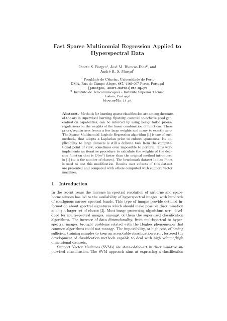
Fig. 1. Evolution of energy (9) when computed with (12) and with the Block Gauss-
Seidel iterative scheme proposed in [12]. Notice the huge difference in time for a problem
with n = 500, d = 500, and m = 9. FSMRL takes 8 seconds, whereas SMRL takes 320
seconds.
Figure 1 illustrates the gain in computational cost of the proposed fast SMLR
(FSMRL) for a problem with n = 500, d = 500, and m = 9 on a 2GHz PC. Only
the first ten iterations are shown. Notice that for a very similar energy, SMRL
takes 320 seconds, whereas FSMRL takes 8 seconds.

6 Janete S. Borges et al.
3 Experimental Results
3.1 Data Description
Experiments are performed with an AVIRIS spectrometer image, the Indian
Pines 92 from Northern Indiana, taken on June 12, 1992 [15]. The ground truth
data image consists of 145 x 145 pixels of the AVIRIS image in 220 contiguous
spectral bands, at 10 nm intervals in the spectral region from 0.40 to 2.45 µm,
at a spatial resolution of 20 m. Four of the 224 original AVIRIS bands contained
no data or zero values and were thus removed. The image covers an agricultural
portion of North-West Indiana with 16 identified classes. Due to the insufficient
number of training samples, seven classes were discarded, leaving a dataset with
9 classes distributed by 9345 elements. This dataset was randomly divided into
a set of 4757 training samples and 4588 validation samples. The number of
samples per class and the class labels are presented in table 1 and their spatial
distribution in figure 2.
Fig. 2. AVIRIS image used for testing. Left: original image band 50 (near infrared);
Centre: training areas; Right: validation areas.
Table 1. Number of training and validation samples used in the experiments
Class
Training Validation
C1 - Corn-no till 742 692
C2 - Corn-min till 442 392
C3 - Grass/Pasture 260 237
C4 - Grass/Trees 389 358
C5 - Hay-windrowed 236 253
C6 - Soybean-no till 487 481
C7 - Soybean-min till 1245 1223
C8 - Soybean-clean till 305 309
C9 - Woods 651 643

Lecture Notes in Computer Science 7
3.2 Experimental Setup
Two different types of classifiers using linear and RBF kernels were evaluated in
different conditions: (i)using 10%, 20% and 100% of the training samples to learn
a linear kernel, (ii) using 10%, 20% and 50% of the training samples to learn a
RBF kernel. The six classifiers were applied to (i) the entire set of bands, and
(ii) discarding 20 noisy bands (104-108, 150-163, 220), resulting on 12 scenarios.
These noisy bands correspond to the spectral regions where there is significant
absorption of radiation by the atmosphere due to water vapour. The two types
of classifiers have parameters that are defined by the user. In the case of linear
kernel, only the λ parameter has to be tuned. Together with λ, the RBF kernel
has also the parameter σ that should be tuned.
The tuning process was done by first dividing the training set into a subset
with approximately 10% of training samples, which was used to learn the classifier,
and the remaining 90% used to compute an estimate of the Overall Accuracy
(OA). This process was repeated 20 times in order to obtain the parameter that
maximizes the OA in the remaining training sets. Since the RBF kernel had
two parameters to be tuned, we first looked for the best σ in one subset and
then repeated the same process using the σ achieved. Several values for λ and σ
were tested: for the linear kernel λ = 16, 18, 20, 22, 24; for the RBF kernel
λ = 0.0004,0.00045,0.0005,0.00055,0.0006 and σ = 0.48,0.54,0.6,0.66,0.72.
Table 2. Overall accuracy of a RBF kernel classification, measured on a subset of the
training dataset.
λ/σ 0.48 0.54 0.6 0.66 0.72
0.0004 85.06% 85.53% 85.37% 84.93% 84.40%
0.00045 85.14% 85.56% 85.32% 84.98% 84.38%
0.0005 85.24% 85.50% 85.32% 84.82% 84.27%
0.00055 85.45% 85.43% 85.22% 84.66% 84.43%
0.0006 85.48% 85.40% 84.95% 84.56% 84.38%
In table 2 an example of the tuning process over one subset of 20% of the
training samples and 220 spectral bands is showed. In this example we take
σ = 0.00054 as the best σ. Then we fixed this value and looked for the best
λ running 20 times the same procedure for different subsets of the same size.
The same process was carried out to achieve the best λ and σ using 10% of the
training set for RBF kernel.
When dealing with the complete training set and linear kernel, a crossvalidation
procedure was performed for λ = 16, 18, 20, 22, 24. The implementation
of the method presented was done in Matlab [16], which unfortunately
has several limitations when dealing with large datasets. Therefore, it was not
possible to perform the learning task with a RBF kernel using the complete
training set. In the case of RBF kernel, only 50% of the training samples were

8 Janete S. Borges et al.
used. The best parameters identified by subsets with 20% of training samples
were selected to perform a classification with RBF kernel over the validation
dataset.
3.3 Results
The results presented in this section are the overall accuracy measure in the
independent (validation) dataset with 4588 samples. In tables 3 and 4, the parameters
used for each experimental scenario and respective number of support
vectors are presented. As one can see, there is in fact a large reduction on the
number of features needed to built the classifier. In the case of linear kernel, and
using the entire training set, we can see a significant reduction of the number of
training samples required to build the classifier. In the RBF case, the reduction
is not so great but it is still meaningful.
Table 3. Best λ and number of support vectors (SV) used with linear kernel.
220 Bands 200 Bands
10% 20% 100% 10% 20% 100%
λ 16 22 18 16 18 18
SV 28 22 85 24 39 37
Table 4. Best λ and σ and number of support vectors (SV) used with RBF kernel.
220 Bands 200 Bands
10% 20% 10% 20%
λ 0.0005 0.0006 0.0004 0.0006
σ 0.72 0.54 0.48 0.6
SV 410 689 570 748
Knowing that 20 of the 220 original spectral bands are noisy bands, experiments
were carried out with and without those bands. The objective was to
observe the influence of a coarse feature selection on the classifiers performance.
Tables 5 and 6 present the OA(%) for each case. The improvement in OA due
to the coarse selection is not significant. In some cases, the use of all 220 bands
gives better results than with 200 bands (without the noisy bands). However, it
is worth noting that the differences are not significant in both cases.
In order to better evaluate our results, a comparison was made with the
results obtained with other kernel-based methods in the same dataset [4]. Al-

Lecture Notes in Computer Science 9
Table 5. Results with linear kernel using 10%, 20% and the complete training set.
10% 20% 100%
220 bands 76.55% 79.69% 85.77%
200 bands 75.57% 81.60% 85.24%
Table 6. Results with RBF kernel using 10%, 20% and 50% of training samples.
10% 20% 50%
220 bands 82.93% 87.12% 90.12%
200 bands 84.98% 86.73% 90.52%
though there were some limiting factors in the pratical application of the proposed
method, due to limitations in Matlab processing capacity, the results obtained
are very encouraging. The performance of FSMLR linear proved to be
superior to Linear Discriminant Analysis (LDA) [4] as it is summarised in table
7. Regarding the use of RBF kernels, our results are about the same as those from
[4]. The values presented in 7 for SVM-RBF are approximate values extracted
from graphical data presented in figure 6 of [4]. Although for RBF kernels our
method did not outperform the method used in [4], the sparsity of FSMLR can
be an advantage for large datasets.
Table 7. Comparison of the proposed method with the results from [4].
SMLR Linear LDA [4] SMLR RBF (50%) SVM-RBF (50%) [4]
220 bands 85.77% 82.32% 90.12% ≃ 91%
200 bands 85.24% 82.08% 90.52% ≃ 91%
4 Conclusion
In this work the Block Gauss-Seidel method for solving systems is introduced
in the SMLR classification algorithm. This approach turns the SMLR a faster
and more efficient algorithm for the classification of hyperspectral images. The
performance of this technique was tested using a benchmarked dataset (Indian
Pines) with nine classes and thousands of labelled samples.
Although the experiments performed in this work were suboptimal, the results
proved to be quite satisfactory when compared with the ones achieved by
Camps-Valls et. al [4]. Results with linear kernels were better than the ones

10 Janete S. Borges et al.
achieved with LDA method in [4]. Approximately the same results for RBF kernels
were obtained with our method and by Camps-Valls [4], using only 50% of
the dataset and without tuning all the parameters.
The preliminary results presented in this paper are encouraging as a starting
point for the inclusion of statistical spatial information in classification of hyperspectral
images. Future work can be developed to include the spatial context,
in the sense that neighbouring labels are more likely to have similar labelling.
Plans for future work also include the development of semi-supervised techniques
based on the FSMLR method proposed.
5 Acknoledgments
The first author would like to thank the Fundação para a Ciência e a Tecnologia
(FCT) for the financial support (PhD grant SFRH/BD/17191/2004). The
authors would also like to thank David Landgrebe for providing the AVIRIS
data.
References
1. Krishnapuram, B. Carin, L. Figueiredo, M.A.T. and Hartemink, A.J.: Sparse
Multinomial Logistic Regression: Fast Algorithms and Generalization Bounds. IEEE
Transactions on Pattern Analysis and Machine Intelligence, Vol. 27, Issue 6. (2005)
957-968.
2. Landgrebe, D.A. : Signal Theory Methods in Multispectral Remote Sensing. John
Wiley and Sons, Inc., Hoboken, New Jersey. (2003)
3. Vapnik, V. : Statistical Learning Theory. John Wiley, New York. (1998)
4. Camps-Valls, G. and Bruzzone, L. : Kernel-based methods for hyperspectral image
classification. IEEE Transactions on Geoscience and Remote Sensing, Vol. 43, Issue
6. (2005) 1351–1362.
5. Tipping, M. : Sparse Bayesian learning and the relevance vector machine. Journal
of Machine Learning Research, Vol. 1. (2001) 211–244.
6. Figueiredo, M. : Adaptive Sparseness for Supervised Learning. IEEE Transactions
on Pattern Analysis and Machine Intelligence, Vol. 25, no. 9. (2003) 1150–1159.
7. Csato, L. and Opper, M. : Sparse online Gaussian processes. Neural Computation,
Vol. 14, no. 3. (2002) 641–668.
8. Lawrence, N.D. Seeger, M. and Herbrich, R.: Fast sparse Gaussian process methods:
The informative vector machine. In: Becker, S. Thrun, S. and Obermayer, K. (eds.):
Advances in Neural Information Processing Systems 15. MIT Press, Cambridge,
M.A. (2003) 609–616.
9. Krishnapuram, B. Carin, L. and Hartemink, A.J.: Joint classifier and feature optimization
for cancer diagnosis using gene expression data. Proceedings of th International
Conference in Research in Computational Molecular Biology (RECOMB’03)
Berlin, Germany (2003).
10. Krishnapuram, B. Carin, L. Hartemink, A.J. and Figueiredo, M.A.T. : A Bayesian
approach to joint feature selection and classifier design. IEEE Transactions on Pattern
Analysis and Machine Intelligence, Vol. 26. (2004) 1105-1111.

Lecture Notes in Computer Science 11
11. A.Quarteroni, R.Sacco and F.Saleri: Numerical Mathematics. Springer-Verlag,
New-York. (2000)TAM Series n. 37..
12. Bioucas Dias, J.M. : Fast Sparse Multinomial Logistic Regression - Technical Report.
Instituto Superior Técnico. Available at http://www.lx.it.pt/˜bioucas/ (2006).
13. Hastie, T., R. Tibshirani, and J. Friedman: The Elements of Statistical Learning -
Data Mining, Inference and Prediction. Springer, New York. (2001).
14. Lange, K., Hunter, D. and Yang, I. : Optimizing transfer using surrogate objective
functions. Journal of Computational and Graphical Statistics, Vol. 9. (2000) 1–59.
15. Landgrebe, D.A. : NW Indiana’s Indian Pine (1992). Available at
http://dynamo.ecn.purdue.edu/˜biehl/MultiSpec/.
16. The MathWorks : MATLAB The Language of Technical Computing - Using MAT-
LAB : version 6. The Math Works, Inc. (2000)