doppler evaluation of valvular stenosis #3 - Echo in Context
doppler evaluation of valvular stenosis #3 - Echo in Context
doppler evaluation of valvular stenosis #3 - Echo in Context

Create successful ePaper yourself
Turn your PDF publications into a flip-book with our unique Google optimized e-Paper software.
DOPPLER EVALUATION OF VALVULAR STENOSIS <strong>#3</strong><br />
Joseph A. Kisslo, MD<br />
David B. Adams, RDCS<br />
INTRODUCTION<br />
One reason for the rapid growth <strong>in</strong> the use <strong>of</strong> Doppler echocardiography is its utility <strong>in</strong> detect<strong>in</strong>g<br />
and assess<strong>in</strong>g the severity <strong>of</strong> <strong>valvular</strong> <strong>stenosis</strong>. Detection <strong>of</strong> the presence <strong>of</strong> stenotic <strong>valvular</strong> heart<br />
disease us<strong>in</strong>g Doppler echocardiography was orig<strong>in</strong>ally described over ten years ago. It has<br />
subsequently been demonstrated that Doppler blood velocity data could be used to estimate the<br />
severity <strong>of</strong> a stenotic lesion.<br />
FORWARD BLOOD FLOW PROFILES<br />
Aortic Valve Flow Velocity Pr<strong>of</strong>iles<br />
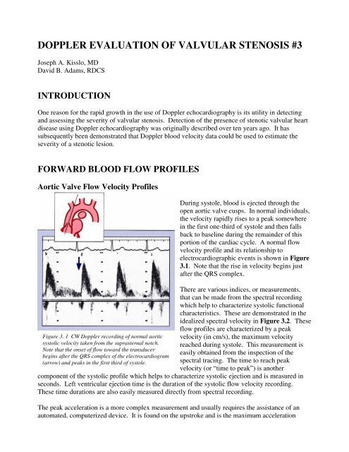
Figure 3. 1 CW Doppler record<strong>in</strong>g <strong>of</strong> normal aortic<br />
systolic velocity taken from the suprasternal notch.<br />
Note that the onset <strong>of</strong> flow toward the transducer<br />
beg<strong>in</strong>s after the QRS complex <strong>of</strong> the electrocardiogram<br />
(arrow) and peaks <strong>in</strong> the first third <strong>of</strong> systole.<br />
Dur<strong>in</strong>g systole, blood is ejected through the<br />
open aortic valve cusps. In normal <strong>in</strong>dividuals,<br />
the velocity rapidly rises to a peak somewhere<br />
<strong>in</strong> the first one-third <strong>of</strong> systole and then falls<br />
back to basel<strong>in</strong>e dur<strong>in</strong>g the rema<strong>in</strong>der <strong>of</strong> this<br />
portion <strong>of</strong> the cardiac cycle. A normal flow<br />
velocity pr<strong>of</strong>ile and its relationship to<br />
electrocardiographic events is shown <strong>in</strong> Figure<br />
3.1. Note that the rise <strong>in</strong> velocity beg<strong>in</strong>s just<br />
after the QRS complex.<br />
There are various <strong>in</strong>dices, or measurements,<br />
that can be made from the spectral record<strong>in</strong>g<br />
which help to characterize systolic functional<br />
characteristics. These are demonstrated <strong>in</strong> the<br />
idealized spectral velocity <strong>in</strong> Figure 3.2. These<br />
flow pr<strong>of</strong>iles are characterized by a peak<br />
velocity (<strong>in</strong> cm/s), the maximum velocity<br />
reached dur<strong>in</strong>g systole. This measurement is<br />
easily obta<strong>in</strong>ed from the <strong>in</strong>spection <strong>of</strong> the<br />
spectral trac<strong>in</strong>g. The time to reach peak<br />
velocity (or “time to peak”) is another<br />
component <strong>of</strong> the systolic pr<strong>of</strong>ile which helps to characterize systolic ejection and is measured <strong>in</strong><br />
seconds. Left ventricular ejection time is the duration <strong>of</strong> the systolic flow velocity record<strong>in</strong>g.<br />
These time durations are also easily measured directly from spectral record<strong>in</strong>g.<br />
The peak acceleration is a more complex measurement and usually requires the assistance <strong>of</strong> an<br />
automated, computerized device. It is found on the upstroke and is the maximum acceleration
expressed <strong>in</strong> centimeters per second. Likewise, measurement <strong>of</strong> the flow velocity <strong>in</strong>tegral usually<br />
requires computer assistance and is the area<br />
under the spectral flow velocity trac<strong>in</strong>g.<br />
Ejection Rate Indices and Ventricular<br />
Function<br />
Figure 3. 2 Many systolic velocity <strong>in</strong>dices may be<br />
calculated from the flow <strong>in</strong> the ascend<strong>in</strong>g aorta, as<br />
<strong>in</strong>dicated <strong>in</strong> these idealized spectral record<strong>in</strong>gs.<br />
Some <strong>of</strong> these <strong>in</strong>dices relate directly to the<br />
systolic function <strong>of</strong> the left ventricle <strong>in</strong> patients<br />
with normal aortic valves. The better the left<br />
ventricular contraction the more rapid the<br />
acceleration, and the higher the peak velocity.<br />
Conversely, the poorer the left ventricular<br />
ejection (as seen <strong>in</strong> patients with low ejection<br />
fractions), the less rapid the acceleration <strong>of</strong><br />
blood flow <strong>in</strong> the aorta and the lower the peak<br />
velocity. These approximate relationships are<br />
illustrated <strong>in</strong> the idealized graphs <strong>in</strong> Figure 3.3.<br />
Thus, rapid peak acceleration and high peak<br />
velocities characterize optimum ejection<br />
fractions.<br />
Cardiac Output<br />
Figure 3. 3 The various ejection rate <strong>in</strong>dices relate to<br />
left ventricular performance (ejection fraction).<br />
Doppler echocardiography is useful for the<br />
determ<strong>in</strong>ation <strong>of</strong> cardiac output; this is the<br />
volume <strong>of</strong> blood pumped by the left ventricle<br />
every m<strong>in</strong>ute and is expressed <strong>in</strong> liters per<br />
m<strong>in</strong>ute. The volume <strong>of</strong> blood ejected every<br />
systolic beat is called the stroke volume (Fig.<br />
3.4) and is the basis for calculation <strong>of</strong> cardiac<br />
output accord<strong>in</strong>g to the follow<strong>in</strong>g equation:<br />
Cardiac output = stroke volume x heart rate<br />
Doppler calculation <strong>of</strong> cardiac output is based<br />
on the assumption that the aorta is a cyl<strong>in</strong>der<br />
dur<strong>in</strong>g every systolic beat. This cyl<strong>in</strong>drical<br />
flow volume may be determ<strong>in</strong>ed if its area and<br />
its length are known. The area is determ<strong>in</strong>ed<br />
from the two-dimensional echocardiographic<br />
image while the length is derived from the<br />
Doppler spectral record<strong>in</strong>g (Fig. 3.5).<br />
Figure 3. 4 Stroke volume is the volume <strong>of</strong> blood<br />
ejected from the left ventricle with each systole.<br />
Know<strong>in</strong>g stroke volume and heart rate provides a<br />
means for calculat<strong>in</strong>g cardiac output. Doppler may be<br />
used for calculat<strong>in</strong>g stroke volume. (CO =cardiac<br />
output; SV = stroke volume; HR=heart rate).<br />
These relationships between area and flow<br />
velocity are shown schematically <strong>in</strong> Figure 3.6.<br />
Given identical volume <strong>of</strong> flow through a large<br />
cyl<strong>in</strong>der (Fig. 3.6, left panel) and small<br />
cyl<strong>in</strong>der (right panel), the velocities recorded<br />
by Doppler will vary considerably. The same<br />
volume through the larger cyl<strong>in</strong>der will render
Figure 3. 5 <strong>Echo</strong>-Doppler estimates <strong>of</strong> flow volume are<br />
based upon a knowledge <strong>of</strong> the area <strong>of</strong> flow (from<br />
echocardiogram) and the length (from Doppler). It is<br />
assumed that the aorta is a cyl<strong>in</strong>der.<br />
a lower peak velocity (and small flow velocity<br />
<strong>in</strong>tegral) <strong>in</strong> comparison with the flow recorded<br />
through the smaller orifice. The flow velocity<br />
<strong>in</strong>tegral reflects the average velocity <strong>of</strong> the red<br />
cells dur<strong>in</strong>g systole. Because the red cells are<br />
mov<strong>in</strong>g faster through the smaller cyl<strong>in</strong>der,<br />
they travel farther. Thus, the Doppler<br />
record<strong>in</strong>g <strong>of</strong> velocity relates to distance<br />
traveled.<br />
Conceptually, derivation <strong>of</strong> cardiac output<br />
beg<strong>in</strong>s with the recognition that the volume <strong>of</strong><br />
blood ejected every time the heart beats is first<br />
limited by the area <strong>of</strong> the aortic root (the area<br />
<strong>of</strong> the cyl<strong>in</strong>der). While there rema<strong>in</strong>s some<br />
argument as to the precise po<strong>in</strong>t where this area<br />
is best determ<strong>in</strong>ed from the two-dimensional echocardiographic image, most Doppler users<br />
measure the narrowest diameter <strong>in</strong> systole at the bases <strong>of</strong> the aortic valve cusps. This is most<br />
reliably accomplished us<strong>in</strong>g the parasternal<br />
long-axis view. Divid<strong>in</strong>g the diameter <strong>in</strong> half<br />
then results <strong>in</strong> the radius <strong>of</strong> the open aortic<br />
valve. This area is assumed to be a circle and<br />
is determ<strong>in</strong>ed by the standard plane geometric<br />
equation: area = r 2 .<br />
Secondly, the distance the ejected blood travels<br />
may be calculated from the Doppler spectral<br />
record<strong>in</strong>g. S<strong>in</strong>ce this is a measure <strong>of</strong> velocity<br />
over time, the flow velocity <strong>in</strong>tegral will result<br />
<strong>in</strong> the average velocity dur<strong>in</strong>g systole.<br />
Figure 3. 6 When stroke volumes are equal and areas<br />
remarkably different, the resultant velocities <strong>of</strong> flow<br />
may be quite different. The velocity for large areas<br />
would be less than for small areas.<br />
As a result <strong>of</strong> know<strong>in</strong>g the average velocity, his<br />
may be normalized for one second and is an<br />
<strong>in</strong>dex <strong>of</strong> how far the blood has traveled. The<br />
method for calculation <strong>of</strong> cardiac output is<br />
demonstrated <strong>in</strong> Figure 3.7.<br />
It is important to recognize that for proper calculation <strong>of</strong> cardiac output us<strong>in</strong>g this approach the<br />
beam must be as parallel to flow as possible.<br />
Alterations <strong>of</strong> a few degrees from parallel will<br />
result <strong>in</strong> lower Doppler velocity record<strong>in</strong>gs and<br />
underestimation <strong>of</strong> cardiac output. Therefore,<br />
aortic outflow is best obta<strong>in</strong>ed from the apical<br />
or suprasternal approaches where the beam is<br />
nearly parallel to normal flow.<br />
Figure 3. 7 Illustration <strong>of</strong> all the steps required for the<br />
calculation <strong>of</strong> cardiac output by Doppler.<br />
It is also important to remember that the<br />
Doppler estimate <strong>of</strong> cardiac output is based on<br />
the square <strong>of</strong> the measured radius <strong>of</strong> the aorta.<br />
Any error <strong>in</strong> this measurement will be<br />
multiplied and may pr<strong>of</strong>oundly affect the<br />
result<strong>in</strong>g calculation.
Figure 3. 8 Idealized representation <strong>of</strong> echo-Doppler<br />
calculations <strong>of</strong> cardiac output compared with that<br />
determ<strong>in</strong>ed by thermodilution.<br />
Doppler estimates <strong>of</strong> cardiac output compare<br />
quite favorably with those obta<strong>in</strong>ed by other<br />
methods. Comparisons have been made with<br />
cardiac output estimated by the Fick pr<strong>in</strong>ciple<br />
at catheterization, with thermodiultion, as well<br />
as with a host <strong>of</strong> other approaches. In general,<br />
these studies show very good correlations,<br />
be<strong>in</strong>g with<strong>in</strong> +10% <strong>of</strong> the other method (Fig.<br />
3.8). Cardiac output may also be determ<strong>in</strong>ed<br />
from flow and diameter measurements through<br />
any <strong>of</strong> the other cardiac valves.<br />
Estimation <strong>of</strong> Pulmonary Arterial<br />
Pressures<br />
Many methods have been proposed for the<br />
estimation <strong>of</strong> pulmonary arterial pressures. Unit 2 discusses the method based on the presence <strong>of</strong><br />
tricuspid regurgitation. Other methods are based on the time to peak velocity <strong>of</strong> the pulmonary<br />
arterial flow velocity record<strong>in</strong>g. These methods only work when there is no evidence for<br />
pulmonary <strong>stenosis</strong>.<br />
Figure 3. 9 Idealized comparisons <strong>of</strong> mean pulmonary<br />
artery (PA) pressure to time-to-peak velocity (left) and<br />
the logarithm <strong>of</strong> mean pulmonary artery pressure to<br />
peak velocity (right).<br />
Methods for estimat<strong>in</strong>g pulmonary arterial<br />
pressures are based on alterations <strong>in</strong> the<br />
capacity <strong>of</strong> the pulmonary vasculature to accept<br />
forward systolic flow. In normal <strong>in</strong>dividuals<br />
without pulmonary hypertension, the<br />
pulmonary vasculature is a very low resistance<br />
circuit and has a great capacity to accept the<br />
sudden <strong>in</strong>crease <strong>in</strong> volume. The vessels are<br />
quite distensible and as blood is ejected from<br />
the right ventricle the time to peak velocity and<br />
acceleration time are accord<strong>in</strong>gly relatively<br />
slow.<br />
In pulmonary hypertension, however, resistance<br />
rises as blood vessels thicken and become less<br />
distensible. This results <strong>in</strong> a dim<strong>in</strong>ished<br />
capacity to accept the forward systolic flow out<br />
<strong>of</strong> the right ventricle. The sudden rush <strong>of</strong> blood <strong>in</strong>to the ma<strong>in</strong> pulmonary artery <strong>in</strong> this sett<strong>in</strong>g<br />
results <strong>in</strong> a more rapid time to peak velocity as well as a more rapid acceleration time.<br />
These relationships are illustrated <strong>in</strong> Figure 3.9, where idealized plots <strong>of</strong> mean pulmonary artery<br />
pressure and time to peak velocity are shown. Note that these relationships are curvil<strong>in</strong>ear, mak<strong>in</strong>g<br />
estimates <strong>of</strong> very high, or very low mean pulmonary pressures difficult. To overcome this problem,<br />
several <strong>in</strong>vestigators have po<strong>in</strong>ted out that plott<strong>in</strong>g time to peak velocity aga<strong>in</strong>st the logarithm <strong>of</strong><br />
the mean pulmonary artery pressures makes the correlations much better.<br />
The cl<strong>in</strong>ical application <strong>of</strong> this approach for estimation <strong>of</strong> mean pulmonary arterial pressure<br />
rema<strong>in</strong>s controversial and many methods have been proposed. Our purpose is to present the<br />
general concept <strong>of</strong> these relationships and the reader should consult current literature for more
detailed descriptions <strong>of</strong> the cont<strong>in</strong>u<strong>in</strong>g<br />
evolution <strong>of</strong> this pr<strong>in</strong>ciple. Many factors must<br />
be taken <strong>in</strong>to account, an important one be<strong>in</strong>g<br />
heart rate. Adult patients with pulmonary<br />
hypertension may have normal heart rates <strong>of</strong><br />
60-70 beats/m<strong>in</strong>, and <strong>in</strong>fants and children >140<br />
beats/m<strong>in</strong>; this may significantly shorten<br />
measurements <strong>of</strong> time to peak velocity or<br />
acceleration times, and affect the reliability <strong>of</strong><br />
these estimates <strong>of</strong> pressure.<br />
Figure 3. 10 Idealized spectral record<strong>in</strong>gs<br />
demonstrat<strong>in</strong>g that time-to-peak velocity is very rapid<br />
<strong>in</strong> patients with pulmonary hypertension.<br />
What is most important is that time to peak<br />
velocity is significantly shortened <strong>in</strong> patients<br />
with pulmonary hypertension. Figure 3.10<br />
demonstrates both normal and rapid time to<br />
peak velocities <strong>in</strong> two idealized spectral<br />
record<strong>in</strong>gs.<br />
ESTIMATION OF THE<br />
SEVERITY OF VALVULAR<br />
STENOSIS<br />
Effect <strong>of</strong> Stenosis on Blood Flow<br />
Figure 3. 11 PW Doppler spectral record<strong>in</strong>g <strong>of</strong> aortic<br />
blood flow (arrow) taken from the apical w<strong>in</strong>dow.<br />
Note the lam<strong>in</strong>ar appearance <strong>of</strong> normal flow. (Scale<br />
marks = 20 cm/s)<br />
Figure 3. 12 Left panel – Without aortic valve<br />
obstruction, systolic pressures are almost the same <strong>in</strong><br />
the ventricle and the aorta. Right panel – When<br />
significant aortic valve obstruction is present, left<br />
ventricular pressure rises much higher than aortic, and<br />
a systolic pressure gradient is present. The size <strong>of</strong> the<br />
arrows represents the magnitude <strong>of</strong> the pressures.<br />
The driv<strong>in</strong>g force for blood to move across any<br />
cardiac valve is the presence <strong>of</strong> a slight<br />
pressure difference normally found between<br />
the chambers (or chamber and great vessel) on<br />
either side <strong>of</strong> the valve. For example, systolic<br />
pressure builds with<strong>in</strong> the left ventricle until it<br />
reaches a po<strong>in</strong>t where it exceeds the pressure<br />
<strong>in</strong> the aorta. The aortic valve is suddenly<br />
thrown open and blood is ejected <strong>in</strong>to the<br />
aorta. In normal <strong>in</strong>dividuals, there is a very<br />
slight (1-2 mmHg) pressure difference between<br />
the left ventricle and aorta that helps drive the<br />
blood across the aortic valve.<br />
Normal aortic valve blood flow is lam<strong>in</strong>ar<br />
(Fig. 3.11) and most <strong>of</strong> the red cells <strong>in</strong> the<br />
aortic root dur<strong>in</strong>g systole are mov<strong>in</strong>g at<br />
approximately the same speed. Graphically,<br />
this translates <strong>in</strong>to a narrow band <strong>of</strong> dark grey<br />
on the pulsed wave (PW) Doppler spectral<br />
record<strong>in</strong>g (Fig. 3 11, arrow). Normal peak<br />
systolic velocity <strong>of</strong> blood flow across the aortic<br />
valve rarely exceeds 1.5 m/s.
Figure 3. 13 CW spectral record<strong>in</strong>g from the apex <strong>in</strong> a<br />
patient with aortic <strong>stenosis</strong>. The velocity spectrum is<br />
broadened and systolic velocity is <strong>in</strong>creased to 4 m/s.<br />
(Scale marks = 2 m/s)<br />
When the aortic valve is diseased, the leaflets<br />
become thickened and progressively lose their<br />
mobility. Eventually, the valve itself becomes<br />
narrowed to the po<strong>in</strong>t where it beg<strong>in</strong>s to<br />
obstruct flow, and aortic <strong>stenosis</strong> is created. In<br />
the presence <strong>of</strong> aortic <strong>stenosis</strong>, systolic pressure<br />
<strong>in</strong> the ventricle must rise high enough to force<br />
the blood across the obstruction <strong>in</strong>to the aorta.<br />
Thus, a pressure drop, or pressure gradient, is<br />
generated (Fig. 3.12). Severe degrees <strong>of</strong> aortic<br />
<strong>stenosis</strong> may result <strong>in</strong> aortic valve gradients<br />
that exceed 100 mmHg <strong>in</strong> systole. As<br />
discussed <strong>in</strong> Unit 1, the presence <strong>of</strong> such an<br />
obstruction results <strong>in</strong> both turbulent flow and<br />
<strong>in</strong>creased velocity, two characteristics readily<br />
detected by Doppler echocardiography.<br />
Because <strong>of</strong> the large gradient, the pressures<br />
with<strong>in</strong> the left ventricle rise significantly and<br />
left ventricular hypertrophy results.<br />
Doppler detection and <strong>evaluation</strong> <strong>of</strong> the<br />
presence or absence <strong>of</strong> aortic <strong>stenosis</strong> is based<br />
on record<strong>in</strong>g turbulence and <strong>in</strong>creased flow<br />
velocity <strong>in</strong> the ascend<strong>in</strong>g aorta. In Figure 3.13<br />
these characteristics are shown <strong>in</strong> a cont<strong>in</strong>uous<br />
wave (CW) spectral velocity record<strong>in</strong>g <strong>of</strong><br />
aortic systolic flow obta<strong>in</strong>ed from the apical<br />
w<strong>in</strong>dow. Turbulent flow is represented by<br />
broaden<strong>in</strong>g <strong>of</strong> the velocity spectrum. There is<br />
also an <strong>in</strong>crease <strong>in</strong> peak aortic velocity to 4<br />
m/s. The Doppler audio <strong>in</strong> this case had a<br />
harsh, higher pitched quality dur<strong>in</strong>g systole<br />
that was easily dist<strong>in</strong>guished from the sound <strong>of</strong><br />
lam<strong>in</strong>ar flow.<br />
Figure 3. 14 CW Doppler spectral velocity record<strong>in</strong>g<br />
<strong>of</strong> mild pulmonic <strong>stenosis</strong> and <strong>in</strong>sufficiency. The<br />
abnormal diastolic flow toward the transducer <strong>of</strong><br />
pulmonic <strong>in</strong>sufficiency is easily recognized. (Scale<br />
marks = 1m/s)<br />
Similarly, the presence <strong>of</strong> these characteristics<br />
<strong>in</strong> the pulmonary artery dur<strong>in</strong>g systole would<br />
<strong>in</strong>dicate the presence <strong>of</strong> obstruction to right<br />
ventricular ejection. Figure 3.14 demonstrates<br />
a CW Doppler spectral record<strong>in</strong>g from the left<br />
parasternal w<strong>in</strong>dow <strong>in</strong> a patient with mild<br />
pulmonic <strong>stenosis</strong> and <strong>in</strong>sufficiency. Turbulent<br />
diastolic and systolic flows are noted with a<br />
slight <strong>in</strong>crease <strong>in</strong> the peak systolic velocity to<br />
1.4 m/s (normal
turbulent and the peak systolic velocity is<br />
elevated. The spectral record<strong>in</strong>g <strong>of</strong> pulmonic<br />
<strong>in</strong>sufficiency is lost because the sample volume<br />
is located distal to this lesion.<br />
While PW Doppler is very useful for the<br />
localization <strong>of</strong> such obstructive lesions, it has<br />
limited value <strong>in</strong> establish<strong>in</strong>g the severity <strong>of</strong><br />
obstruction because most significant <strong>valvular</strong><br />
obstructions result <strong>in</strong> velocities above 1.5 m/s.<br />
As emphasized previously, velocities above 1.5<br />
m/s will usually cause alias<strong>in</strong>g <strong>of</strong> the PW<br />
record<strong>in</strong>g. This prevents the faithful record<strong>in</strong>g<br />
<strong>of</strong> peak velocities necessary for the calculation<br />
<strong>of</strong> valve gradients.<br />
Figure 3. 15 PW Doppler spectral record<strong>in</strong>g from the<br />
same patient as Figure 3.24. At position A, pulmonic<br />
<strong>in</strong>sufficiency is noted. At position B, on the distal side<br />
<strong>of</strong> the valve, the systolic velocity is elevated. (Scale<br />
marks = 20cm/s)<br />
Estimation <strong>of</strong> the Severity <strong>of</strong> Stenosis<br />
Use <strong>of</strong> Doppler ultrasound to estimated the<br />
severity <strong>of</strong> a valve <strong>stenosis</strong> is based pr<strong>in</strong>cipally<br />
on the fact that such obstructions result <strong>in</strong> an<br />
<strong>in</strong>crease <strong>in</strong> the velocity <strong>of</strong> flow. In cl<strong>in</strong>ically<br />
significant mitral <strong>stenosis</strong>, the diastolic velocity<br />
<strong>of</strong> mitral flow usually exceeds 1.7 m/s. Systolic<br />
velocity <strong>of</strong> aortic flow <strong>in</strong> cl<strong>in</strong>ically significant<br />
aortic <strong>stenosis</strong> may reach 5-6 m/s (Fig. 3.16).<br />
Thus, CW Doppler is required for the detection<br />
<strong>of</strong> these <strong>in</strong>creased velocities and for record<strong>in</strong>g<br />
the full spectral pr<strong>of</strong>iles.<br />
Figure 3. 16 Typical CW spectral velocity trac<strong>in</strong>g from<br />
the apex <strong>in</strong> a patient with aortic <strong>stenosis</strong> and<br />
<strong>in</strong>sufficiency. Peak systolic velocity is elevated to<br />
almost 6 m/s and peak<strong>in</strong>g is delayed. (Scale marks = 2<br />
m/s)<br />
We have already noted that there is a<br />
relationship between the pressure <strong>in</strong>crease (or<br />
gradient) across a valve and the velocity <strong>of</strong><br />
blood flow across the valve. For any given<br />
pressure gradient there is a correspond<strong>in</strong>g<br />
<strong>in</strong>crease <strong>in</strong> velocity, as predicted by the<br />
simplified Bernoulli equation:<br />
p 1 -p 2 = 4V 2<br />
where p 1 = pressure distal to obstruction p 2 =<br />
peak velocity <strong>of</strong> blood flow across the<br />
obstruction.<br />
As the <strong>stenosis</strong> becomes more severe, the valve<br />
orifice area will become smaller, and the velocity <strong>of</strong> flow across the orifice will <strong>in</strong>crease as a<br />
function <strong>of</strong> the <strong>in</strong>creased pressure gradient. Thus, by measur<strong>in</strong>g the peak velocity <strong>in</strong> a systolic<br />
aortic jet with Doppler echocardiography, it is possible to estimate the pressure gradient that<br />
produced it us<strong>in</strong>g the above simple algebraic expression. The peak aortic velocity <strong>of</strong> the spectral<br />
record<strong>in</strong>g <strong>in</strong> Figure 3.16 is approximately 5.8 m/s. Us<strong>in</strong>g the previous formula<br />
p 1 -p = 4(5.8) 2
the pressure gradient is therefore 135 mmHg.<br />
Figure 3. 17 Idealized relationship between pressure<br />
gradient and flow. As flow <strong>in</strong>creases, the gradient will<br />
also rise even though the valve area is fixed<br />
There are, however, three major technical<br />
requirements that must be satisfied if Doppler<br />
is to be used for this purpose. First, an<br />
adequate “w<strong>in</strong>dow” <strong>in</strong>to the chest for<br />
ultrasound propagation and reception must be<br />
found so that well formed Doppler pr<strong>of</strong>iles can<br />
be recorded. Second, as emphasized <strong>in</strong> Units 1<br />
and 2, for the velocity measurement to be<br />
accurate, this w<strong>in</strong>dow must allow orientation <strong>of</strong><br />
the ultrasound beam so that it is as parallel as<br />
possible to flow through the valve. Third, the<br />
high velocities present <strong>in</strong> the disturbed jet <strong>of</strong>ten<br />
exceed the Nyquist limit <strong>of</strong> PW Doppler, so<br />
that CW or high pulse repetition frequency<br />
Doppler must be used.<br />
Express<strong>in</strong>g the Severity <strong>of</strong> Stenosis<br />
It should be recognized that knowledge <strong>of</strong> the gradient across a stenotic valve does not provide all<br />
the <strong>in</strong>formation necessary to assess the severity <strong>of</strong> obstruction. The gradient will vary with flow<br />
across the stenotic valve orifice and will <strong>in</strong>crease <strong>in</strong> high flow situations and decrease <strong>in</strong> low flow<br />
situations. Thus, a patient with a fixed valve area will have a higher gradient dur<strong>in</strong>g exercise when<br />
cardiac output is <strong>in</strong>creased, than at rest when cardiac output is lower. Figure 3.17 shows the<br />
idealized relationship <strong>of</strong> valve gradient to flow. As flow across a valve rises, as with rapid<br />
tachycardia, the gradients will vary.<br />
Valve orifice size is generally considered not to vary with the amount <strong>of</strong> flow across the valve and<br />
is, therefore, a preferred expression <strong>of</strong> the severity <strong>of</strong> a given <strong>stenosis</strong>. The follow<strong>in</strong>g discussion<br />
will beg<strong>in</strong> with estimates <strong>of</strong> gradients across stenotic valves and then review some <strong>of</strong> the simplified<br />
methods for estimat<strong>in</strong>g valve orifice area.<br />
F<strong>in</strong>d<strong>in</strong>g the Stenotic Jet<br />
Figure 3. 18 CW Doppler spectral record<strong>in</strong>g <strong>of</strong> aortic<br />
outflow from the suprasternal notch with flow toward<br />
the transducer (left) and apex with flow away form the<br />
transducer (right). The spectral record<strong>in</strong>g from the<br />
apex is better formed than the one from the<br />
suprasternal notch.<br />
The most common w<strong>in</strong>dows utilized for<br />
record<strong>in</strong>g peak aortic systolic velocity are the<br />
apical, suprasternal, and right parasternal.<br />
While stenotic jets, like regurgitant jets, are<br />
<strong>of</strong>ten directed eccentrically, it is usually<br />
possible to f<strong>in</strong>d a fully formed aortic systolic<br />
pr<strong>of</strong>ile from one <strong>of</strong> these w<strong>in</strong>dows. A<br />
comprehensive Doppler exam<strong>in</strong>ation for aortic<br />
<strong>stenosis</strong> requires that the ascend<strong>in</strong>g aorta be<br />
exam<strong>in</strong>ed from all possible w<strong>in</strong>dows <strong>in</strong> order to<br />
align the beam parallel to the jet. Figure 3.18<br />
shows a CW exam<strong>in</strong>ation <strong>of</strong> a patient with<br />
aortic <strong>stenosis</strong> from the suprasternal notch (left<br />
panel) and the apex (right panel). The<br />
spectral trac<strong>in</strong>g from the apical w<strong>in</strong>dow is
superior as judged by the presence <strong>of</strong> a fully<br />
formed pr<strong>of</strong>ile with a discrete ascent, peak, and<br />
descent. While we have found the apical<br />
w<strong>in</strong>dow to be most productive, we always<br />
exam<strong>in</strong>e the aorta from every possible view.<br />
Occasionally, the suprasternal w<strong>in</strong>dow will be<br />
perfectly aligned to flow and will present the<br />
typical spectral pr<strong>of</strong>ile <strong>of</strong> aortic <strong>stenosis</strong>. This<br />
is demonstrated <strong>in</strong> a patient with severe aortic<br />
<strong>stenosis</strong> <strong>in</strong> Figure 3.19. In this condition, there<br />
is marked spectral broaden<strong>in</strong>g, delayed systolic<br />
peak<strong>in</strong>g, and a marked <strong>in</strong>crease <strong>in</strong> velocity. In<br />
this patient, the peak systolic velocity is almost<br />
5 m/s (100mmHg).<br />
Figure 3. 19 Typical aortic systolic velocity record<strong>in</strong>g<br />
from the suprasternal notch <strong>in</strong> a patient with aortic<br />
<strong>stenosis</strong>. Note that the peak velocity is almost 5 m/s.<br />
As gradient <strong>in</strong>creases, so does the peak systolic<br />
velocity. (Scale marks = 1m/s)<br />
Figure 3. 20 Operator skill is important <strong>in</strong> obta<strong>in</strong><strong>in</strong>g<br />
an adequate systolic aortic jet pr<strong>of</strong>ile <strong>in</strong> aortic <strong>stenosis</strong>.<br />
This figure shows a record<strong>in</strong>g made by a less<br />
experienced operator (left panel) compared with one<br />
from a more experienced operator (right panel).<br />
Considerable operator skill is required to obta<strong>in</strong><br />
adequate spectral trac<strong>in</strong>gs for measurement <strong>of</strong><br />
peak velocity. It is our experience that the<br />
Doppler exam<strong>in</strong>ation for aortic <strong>stenosis</strong> will<br />
add an average <strong>of</strong> 15-30 m<strong>in</strong>utes to the twodimensional<br />
and rout<strong>in</strong>e Doppler<br />
echocardiographic exam<strong>in</strong>ation, even with the<br />
experienced operator.<br />
In Figure 3.20 (left panel) there is a record<strong>in</strong>g<br />
from the apical w<strong>in</strong>dow obta<strong>in</strong>ed by an operator<br />
with only modest experience. Both aortic<br />
<strong>stenosis</strong> and aortic <strong>in</strong>sufficiency are recorded,<br />
but the systolic flow away form the transducer<br />
fails to show a fully formed pr<strong>of</strong>ile. The<br />
spectral record<strong>in</strong>g <strong>in</strong> Figure 3.20 (right panel)<br />
was performed by a more experienced<br />
<strong>in</strong>dividual, and the fully formed systolic pr<strong>of</strong>ile<br />
is seen. Had a measurement been made on the<br />
upper panel, peak systolic velocity would have<br />
been approximately 2.8 m/s, while the true<br />
velocity shown on the panel below is 5 m/s.<br />
Use <strong>of</strong> the <strong>in</strong>adequate trac<strong>in</strong>g would have<br />
severely underestimated the valve gradient.<br />
Most experienced Doppler operators can obta<strong>in</strong><br />
aortic systolic velocity pr<strong>of</strong>iles adequate for<br />
measurement <strong>of</strong> peak velocity <strong>in</strong> about 95% <strong>of</strong><br />
patients. Figure 3.21 demonstrates comb<strong>in</strong>ed<br />
aortic <strong>stenosis</strong> and <strong>in</strong>sufficiency by CW<br />
Doppler from the apex <strong>of</strong> the left ventricle.<br />
Note that at the left, the full pr<strong>of</strong>ile <strong>of</strong> the aortic<br />
stenotic jet is encountered. With m<strong>in</strong>imum<br />
transducer angulation, the aortic <strong>in</strong>sufficiency<br />
Figure 3. 21 The systolic jet <strong>of</strong> aortic <strong>stenosis</strong> and diastolic jet <strong>of</strong> aortic <strong>in</strong>sufficiency <strong>of</strong>ten cannot be recorded at the<br />
same time. As the transducer beam is angled from the stenotic jet (closed arrow) to <strong>in</strong>tercept the aortic <strong>in</strong>sufficiency, the<br />
left ventricular outflow tact velocity is encountered (stippled arrow). Both outflow tract velocities are superimposed<br />
dur<strong>in</strong>g the beam sweep (open arrow). (Scale marks = 1m/s)
pr<strong>of</strong>ile is readily encountered. At the far right,<br />
the systolic flow away from the transducer is<br />
lower <strong>in</strong> velocity and represents the velocity <strong>in</strong><br />
the left ventricular outflow tract before the<br />
obstruction. The lower velocity proximal to the<br />
stenotic valve should not be confused with<br />
aortic <strong>stenosis</strong>.<br />
Figure 3. 22 Inadequate record<strong>in</strong>gs <strong>of</strong> aortic systolic<br />
velocity do occur and should not be used for estimation<br />
<strong>of</strong> gradient. Note that the pr<strong>of</strong>ile is poorly formed on<br />
the upstroke, peak (arrow), and down stroke. (Scale<br />
marks = 2 m/s)<br />
Figure 3. 23 Aortic <strong>stenosis</strong> (left) should not be<br />
mistaken for mitral <strong>in</strong>sufficiency (right). Mitral systole<br />
beg<strong>in</strong>s before aortic (arrow) and is longer <strong>in</strong> duration.<br />
(Scale marks = 2m/s)<br />
Figure 3. 24 Relationship between abnormal systolic<br />
and diastolic flows through the left heart valves. For<br />
details, see text.<br />
Occasionally, only <strong>in</strong>completely formed<br />
pr<strong>of</strong>iles are recorded. These should be<br />
considered <strong>in</strong>adequate and never used for<br />
estimation <strong>of</strong> gradient. An <strong>in</strong>completely<br />
formed pr<strong>of</strong>ile from an older patient is shown<br />
<strong>in</strong> Figure 3.22.<br />
Another potential source for error is mistakenly<br />
<strong>in</strong>terpret<strong>in</strong>g the pr<strong>of</strong>ile <strong>of</strong> mitral <strong>in</strong>sufficiency<br />
for that <strong>of</strong> aortic <strong>stenosis</strong>. When recorded from<br />
the apical w<strong>in</strong>dow, both occur <strong>in</strong> systole and<br />
are displayed as downward spectral velocity<br />
shifts. This is seen <strong>in</strong> the spectral trac<strong>in</strong>gs<br />
shown <strong>in</strong> Figure 3.23. These may be<br />
differentiated by remember<strong>in</strong>g that the onset <strong>of</strong><br />
ventricular systole and mitral regurgitation<br />
(3.23 arrow) occurs prior to aortic valve<br />
open<strong>in</strong>g. In addition, mitral regurgitation is<br />
longer <strong>in</strong> duration.<br />
At first, it may appear that the spectral pr<strong>of</strong>iles<br />
<strong>of</strong> aortic <strong>stenosis</strong> resemble mitral <strong>in</strong>sufficiency<br />
and those <strong>of</strong> aortic <strong>in</strong>sufficiency resemble<br />
mitral <strong>stenosis</strong>. These disease pr<strong>of</strong>iles may be<br />
differentiated by a knowledge <strong>of</strong> the various<br />
tim<strong>in</strong>g relationships <strong>of</strong> left-sided <strong>valvular</strong><br />
open<strong>in</strong>g and clos<strong>in</strong>g. Figure 3.24 shows the<br />
relationships between these various abnormal<br />
spectral velocities. The duration <strong>of</strong> mitral<br />
<strong>in</strong>sufficiency is generally longer than that <strong>of</strong><br />
aortic <strong>stenosis</strong>, partly because the time from<br />
mitral valve clos<strong>in</strong>g to open<strong>in</strong>g is longer than<br />
for aortic valve open<strong>in</strong>g to clos<strong>in</strong>g. Similarly,<br />
the duration <strong>of</strong> aortic <strong>in</strong>sufficiency is longer<br />
than mitral <strong>stenosis</strong> because the time from<br />
aortic valve clos<strong>in</strong>g to open<strong>in</strong>g is longer than<br />
for mitral valve open<strong>in</strong>g to clos<strong>in</strong>g. Similar<br />
relationships are true <strong>of</strong> the pulmonic and<br />
tricuspid valve on the right side <strong>of</strong> the heart.<br />
Those experienced <strong>in</strong> phonocardiography will<br />
realize the advantage <strong>of</strong> us<strong>in</strong>g this technique to<br />
assist <strong>in</strong> the identification <strong>of</strong> the various valve<br />
pr<strong>of</strong>iles.
Figure 3. 25 Left panel shows an aortic stenotic jet <strong>in</strong><br />
relation to possible view<strong>in</strong>g directions us<strong>in</strong>g CW<br />
Doppler. Right panel shows spectral velocity trac<strong>in</strong>gs<br />
from each respective w<strong>in</strong>dow. The best record<strong>in</strong>g is<br />
from the right sternal w<strong>in</strong>dow. (Calibration marks =<br />
2m/s)<br />
Figure 3. 26 CW spectral velocity record<strong>in</strong>g from the<br />
suprasternal w<strong>in</strong>dow <strong>in</strong>to the ascend<strong>in</strong>g aorta from a<br />
patient with severe <strong>stenosis</strong>. Note the vary<strong>in</strong>g peak<br />
velocities with vary<strong>in</strong>g R-R <strong>in</strong>terval <strong>of</strong> the ECG.<br />
(Calibration marks = 1 m/s).<br />
In patients with aortic valve disease and<br />
<strong>stenosis</strong>, a careful exam<strong>in</strong>ation must be<br />
performed from all possible views as the<br />
abnormal jet may be directed anywhere <strong>in</strong> the<br />
aorta. In these cases, we are most <strong>in</strong>terested <strong>in</strong><br />
record<strong>in</strong>g the highest peak systolic velocity<br />
present. As previously po<strong>in</strong>ted out, the most<br />
faithful representation <strong>of</strong> flow will be obta<strong>in</strong>ed<br />
when the beam is parallel. The use <strong>of</strong> multiple<br />
positions for the record<strong>in</strong>g <strong>of</strong> peak systolic<br />
aortic velocity is very important <strong>in</strong> aortic<br />
<strong>stenosis</strong> s<strong>in</strong>ce this jet may be directed <strong>in</strong> a wide<br />
variety <strong>of</strong> orientations. This is especially true<br />
<strong>in</strong> older patients with acquired aortic <strong>stenosis</strong>.<br />
Figure 3.25 demonstrates one such direction <strong>of</strong><br />
flow and its relationship to various transducer<br />
positions for CW Doppler record<strong>in</strong>g. In this<br />
case, peak flow was best recorded by CW<br />
Doppler from the right parasternal approach,<br />
rather than from the suprasternal notch. The<br />
velocity pr<strong>of</strong>ile from the apex seems adequate<br />
but is slightly lower than the right sternal<br />
record<strong>in</strong>g. The record<strong>in</strong>g from the suprasternal<br />
notch is grossly <strong>in</strong>adequate and lacks a fully<br />
formed pr<strong>of</strong>ile. When exam<strong>in</strong><strong>in</strong>g for aortic<br />
<strong>stenosis</strong>, all available acoustic w<strong>in</strong>dows should<br />
be utilized.<br />
There will be times when the chang<strong>in</strong>g<br />
appearance <strong>of</strong> the spectral trace is not the result<br />
<strong>of</strong> an improper beam direction or<br />
misadjustment <strong>of</strong> system controls. Figure 3.26<br />
shows a CW record<strong>in</strong>g from the suprasternal<br />
notch with the beam directed toward the<br />
ascend<strong>in</strong>g aorta. The differ<strong>in</strong>g appearances <strong>of</strong><br />
the velocity pr<strong>of</strong>iles are a result <strong>of</strong> an irregular<br />
heart rate which leads to beat-to-beat changes<br />
<strong>in</strong> stroke volume and, consequently, aortic<br />
gradient. Stenotic jets, like regurgitant jets,<br />
readily change their configuration with cardiac<br />
rhythms.<br />
Aortic Valve Gradient at Catheterization<br />
Estimation <strong>of</strong> trans<strong>valvular</strong> aortic gradients <strong>in</strong> patients with aortic <strong>stenosis</strong> us<strong>in</strong>g Doppler has been<br />
<strong>in</strong> common use for some time. There is an abundance <strong>of</strong> papers <strong>in</strong> the literature discuss<strong>in</strong>g the<br />
relative merits and limitations <strong>of</strong> this approach. All are based upon correlations with pressure<br />
measurements obta<strong>in</strong>ed at catheterization.<br />
In Figure 3.27 three possible methods are shown for calculat<strong>in</strong>g pressure gradients across the aortic<br />
valve at catheterization. All depend upon the record<strong>in</strong>g <strong>of</strong> pressure from the left ventricle and<br />
aorta, or some peripheral artery. If a peripheral artery is used, it takes time for the systolic pulse to
Figure 3. 27 Schematic representation <strong>of</strong> simultaneous<br />
left ventricular (LV) and aortic (Ao) pressure<br />
record<strong>in</strong>gs obta<strong>in</strong>ed at catheterization with<br />
representation <strong>of</strong> different gradient measurement<br />
methods.<br />
be conducted <strong>in</strong>to the aorta and there is usually<br />
a short delay <strong>in</strong> the upstroke <strong>of</strong> the aortic pulse<br />
when compared with that <strong>of</strong> the ventricle. This<br />
requires the <strong>in</strong>dividual measur<strong>in</strong>g these<br />
pressures to trace the aortic pulse and move it<br />
slightly backwards <strong>in</strong> time to adjust for the time<br />
delay. A peak to peak gradient is measured<br />
from the peak <strong>of</strong> the left ventricular pressure<br />
record<strong>in</strong>g to the peak <strong>of</strong> the aortic. Peak<br />
gradient is measured as the largest difference<br />
between the two and occurs somewhere on the<br />
ascend<strong>in</strong>g pressure trac<strong>in</strong>gs. Mean gradient is<br />
estimated by summ<strong>in</strong>g the gradients measured<br />
at sequential time <strong>in</strong>tervals dur<strong>in</strong>g systole and<br />
divid<strong>in</strong>g by the number <strong>of</strong> measurements made.<br />
Appreciation <strong>of</strong> these various <strong>in</strong>vasive methods for calculation <strong>of</strong> the aortic valve gradient is very<br />
important for a critical <strong>in</strong>terpretation <strong>of</strong> the Doppler literature on aortic <strong>stenosis</strong>. Almost all<br />
catheterization laboratories report peak to peak and mean gradients s<strong>in</strong>ce both are readily<br />
performed. Accurate measurement <strong>of</strong> peak gradient, however, is more difficult and requires precise<br />
alignment <strong>of</strong> ventricular and aortic pressures <strong>in</strong> time, and careful search<strong>in</strong>g for the peak, or largest,<br />
<strong>in</strong>stantaneous gradient.<br />
Figure 3. 28 Pressure record<strong>in</strong>gs from the left<br />
ventricle (LV) and brachial artery (BA) from a patient<br />
with aortic <strong>stenosis</strong>. Note the delay <strong>in</strong> the upstroke <strong>of</strong><br />
the brachial arterial pressure trac<strong>in</strong>g and the delay <strong>in</strong><br />
onset <strong>of</strong> the brachial pressure trac<strong>in</strong>g when compared<br />
with that from the ventricle.<br />
Actual left ventricular and brachial arterial<br />
pressure trac<strong>in</strong>gs from a patient with aortic<br />
<strong>stenosis</strong> are shown <strong>in</strong> Figure 3.28. Note that<br />
the rate <strong>of</strong> rise <strong>of</strong> the left ventricular pressure is<br />
much more rapid than that <strong>of</strong> the brachial<br />
artery. Note also that there is a time delay <strong>in</strong><br />
the onset <strong>of</strong> rise <strong>of</strong> the brachial artery. Note<br />
also that there is a time delay <strong>in</strong> the onset <strong>of</strong><br />
rise <strong>of</strong> the brachial arterial pulse. This results<br />
because <strong>of</strong> the time required for the bolus <strong>of</strong><br />
ejected blood to transit the aortic valve and<br />
aorta to the brachial artery. For proper<br />
measurement <strong>of</strong> peak gradient the brachial<br />
pulse must be “set back” to correspond to the<br />
rise <strong>of</strong> the left ventricular pressure trac<strong>in</strong>g.<br />
With the fluid-filled catheters commonly used,<br />
rapid changes <strong>in</strong> pressure, such as occur with<br />
ventricular ejection, occasionally create<br />
overshoot artifacts on the pressure record<strong>in</strong>g.<br />
Peak gradients are <strong>of</strong>ten not reported from catheterization data, <strong>in</strong> part because <strong>of</strong> these artifacts<br />
and tim<strong>in</strong>g delays which can create large measurement errors.<br />
Doppler Estimation <strong>of</strong> Gradient <strong>in</strong> Aortic Stenosis<br />
It is most important to remember that the peak gradient is usually higher than the peak-to-peak or<br />
mean gradients. The spectral record<strong>in</strong>gs result<strong>in</strong>g from Doppler <strong>in</strong>terrogations <strong>of</strong> aortic <strong>stenosis</strong><br />
reflect the highest gradients with<strong>in</strong> the jet. This is frequently referred to as “peak <strong>in</strong>stantaneous<br />
gradient”. Doppler estimates <strong>of</strong> the aortic peak gradient calculated us<strong>in</strong>g the simplified Bernoullis
formula generally overestimate severity when<br />
compared with catheterization peak-to-peak<br />
gradients. Accord<strong>in</strong>gly, Doppler estimates <strong>of</strong><br />
severity would be expected to correlate best<br />
with the peak gradient at catheterization.<br />
Figure 3. 29 Idealized relationship between Doppler<br />
peak gradient and catheterization peak-to-peak<br />
gradient. Comparisons show that there is<br />
overestimation <strong>of</strong> catheterization peak-to-peak<br />
gradient.<br />
In an attempt to evaluate the use <strong>of</strong> Doppler<br />
echocardiography <strong>in</strong> cl<strong>in</strong>ical practice, we<br />
studied sixty consecutive patients who were<br />
referred to the catheterization laboratory with<br />
cl<strong>in</strong>ical f<strong>in</strong>d<strong>in</strong>gs suggestive <strong>of</strong> possible aortic<br />
<strong>stenosis</strong> (aortic systolic murmur and peripheral<br />
pulse deficit). All patients underwent cardiac<br />
catheterization at a time remote from the<br />
Doppler study (usually after 24 hours). The<br />
Doppler exam<strong>in</strong>ation and <strong>in</strong>terpretation was<br />
performed without knowledge <strong>of</strong> the results <strong>of</strong><br />
catheterization. Our patients were older than<br />
many <strong>of</strong> the groups reported from other centers<br />
(mean age 63 years), as one might anticipate <strong>in</strong><br />
rout<strong>in</strong>e cl<strong>in</strong>ical practice, and 45% had a 2+ or<br />
greater aortic <strong>in</strong>sufficiency.<br />
As can be seen <strong>in</strong> Figure 3.29, Doppler over-estimation <strong>of</strong> catheterization peak-to-peak gradient <strong>in</strong><br />
our series was sometimes quite significant. Indeed, overestimations are evident over the entire<br />
spectrum <strong>of</strong> gradient values and vary <strong>in</strong> magnitude between 1 and 53mmHg. In our view, this<br />
f<strong>in</strong>d<strong>in</strong>g suggests that the cl<strong>in</strong>ician must be very careful <strong>in</strong> us<strong>in</strong>g catheterization laboratory criteria<br />
for estimat<strong>in</strong>g the severity <strong>of</strong> an aortic gradient with Doppler peak aortic gradient valves.<br />
Doppler and catheterization estimates are more<br />
comparable when both laboratories report the<br />
peak aortic valve gradient (Fig. 3.30). The<br />
scatter <strong>of</strong> our data is obviously great because<br />
the studies were not performed simultaneously<br />
with catheterization. Altered hemodynamic<br />
states with different volumes <strong>of</strong> blood flow<br />
across the aortic valve could easily account for<br />
the differences between catheterization and<br />
Doppler gradients <strong>in</strong> nonsimultaneous studies.<br />
When Doppler data are collected<br />
simultaneously with catheterization, us<strong>in</strong>g<br />
micromanometer-tipped catheters, the<br />
correlations are much better.<br />
In rout<strong>in</strong>e cl<strong>in</strong>ical practice, Doppler estimates <strong>of</strong><br />
the severity <strong>of</strong> aortic <strong>stenosis</strong> are likely to be made at least 24 hours before catheterization. These<br />
Figure 3. 30 Idealized relationship between Doppler<br />
peak gradient and catheterization peak gradient. S<strong>in</strong>ce<br />
Doppler reflects peak catheterization gradient, the<br />
comparisons are more favorable.<br />
Doppler measurements may f<strong>in</strong>d a role <strong>in</strong><br />
select<strong>in</strong>g patients for <strong>in</strong>vasive study.<br />
Eventually, they may be used to refer some<br />
patients to surgery without prior catheterization.
It is encourag<strong>in</strong>g that even though comparative data were collected at different times <strong>in</strong> our study,<br />
peak gradients correlated favorably. In our experience, if heart rates vary more than 20 beats/m<strong>in</strong><br />
between the two studies, agreement between them will be reduced (due to differences <strong>in</strong> blood flow<br />
across the valve). Therefore, heart rate serves as one convenient <strong>in</strong>dex for assess<strong>in</strong>g the similarity<br />
between hemodynamic states, when Doppler and catheterization comparison studies are performed<br />
at remote times.<br />
Figure 3. 31 Idealized relationship between Doppler<br />
mean gradient and catheterization mean gradient.<br />
Mean gradient comparisons are favorable because they<br />
average data over time.<br />
There are some limitations <strong>in</strong>herent <strong>in</strong> us<strong>in</strong>g<br />
Doppler peak aortic gradient estimates. Few<br />
catheterization laboratories report peak<br />
gradient data, and a suitable frame <strong>of</strong> reference<br />
to judge severity <strong>of</strong> <strong>stenosis</strong> (as exists for peakto-peak<br />
gradients) is not available. Cl<strong>in</strong>icians<br />
have commonly used peak-to-peak gradients <strong>in</strong><br />
excess <strong>of</strong> 50mmHg to identify severe aortic<br />
<strong>stenosis</strong>. There is no correspond<strong>in</strong>g figure for<br />
peak gradients <strong>in</strong> current use.<br />
The comparison <strong>of</strong> mean Doppler gradient with<br />
mean catheterization gradient also shows good<br />
overall agreement (Fig. 3.31). Mean gradients<br />
may be less sensitive to <strong>in</strong>dividual<br />
measurement errors s<strong>in</strong>ce they reflect an<br />
average <strong>of</strong> multiple measurements. The<br />
calculation <strong>of</strong> mean Doppler gradient also has<br />
the advantage that such gradients are available<br />
from most catheterization laboratories and are<br />
familiar to most cl<strong>in</strong>icians. When Doppler and catheterization measurements are collected<br />
simultaneously, the correlations are even better because <strong>of</strong> these factors.<br />
Understand<strong>in</strong>g the details <strong>of</strong> these various gradient comparisons is important for the beg<strong>in</strong>ner to<br />
Doppler echocardiography. We have seen a conflict <strong>of</strong> op<strong>in</strong>ion develop between the<br />
echocardiography and catheterization laboratories when there is not a mutual understand<strong>in</strong>g <strong>of</strong> the<br />
capabilities and limitations <strong>of</strong> both techniques. Despite these cautions, we do believe that Doppler<br />
comparison with catheterization data acquired with pressure transducer-tipped catheters are most<br />
satisfactory when obta<strong>in</strong>ed simultaneously.<br />
Other Aspects <strong>of</strong> Aortic Stenosis<br />
We occasionally encountered patients with a small gradient predicted by Doppler but with no<br />
gradient at catheterization. In most <strong>in</strong>stances, heart rates were nearly identical at the time <strong>of</strong><br />
Doppler and catheterization, mak<strong>in</strong>g it unlikely that differences <strong>in</strong> hemodynamic status were<br />
responsible for the discrepancies. However, it is noteworthy that all <strong>of</strong> these patients had high<br />
cardiac outputs and, <strong>in</strong> most, significant aortic regurgitation was present. It is possible that the use<br />
<strong>of</strong> the simplified Bernoulli equation <strong>in</strong> such patients may be at least partly responsible for the<br />
overestimates. The full Bernoulli equation takes <strong>in</strong>to account blood velocity on both sides <strong>of</strong> the<br />
valve, whereas the simplified form only uses peak velocity after the flow crosses the valve.<br />
In Figure 3.32 the velocity <strong>of</strong> flow on the ventricular side <strong>of</strong> the valve (V 1 ) is simultaneous with<br />
flow <strong>in</strong> the aortic side (V 2 ) us<strong>in</strong>g CW Doppler from the apical approach. Patients with<br />
hyperdynamic circulatory states, such as those with aortic regurgitation, may have a significant<br />
velocity component below the aortic valve. We have also encountered a few patients with very
severe systemic hypertension (with high<br />
peripheral resistance) and high cardiac outputs<br />
where Doppler peak systolic velocities<br />
approached 5 m/s. In each, no gradient was<br />
found at catheterization.<br />
Figure 3. 32 Velocity below the valve (V 1 ) is not<br />
recorded as <strong>of</strong>ten as velocity on the aortic side (V 2 ).<br />
V 1 is ignored <strong>in</strong> the simplified Bernoulli equation.<br />
(Scale marks = 1m/s)<br />
Failure to take these experiences <strong>in</strong>to account<br />
may lead the Doppler operator to attribute the<br />
elevated aortic velocity to an obstruction <strong>of</strong> the<br />
outflow tract, even <strong>in</strong> patients with pure aortic<br />
regurgitation or other reasons for the <strong>in</strong>creased<br />
systolic velocities. In our series, the effect <strong>of</strong><br />
aortic <strong>in</strong>sufficiency was most evident when<br />
there was a m<strong>in</strong>imal or no aortic valve<br />
gradient. It seemed to be less important <strong>in</strong><br />
patients with comb<strong>in</strong>ed <strong>stenosis</strong> and<br />
<strong>in</strong>sufficiency.<br />
Several observations may be helpful <strong>in</strong> recogniz<strong>in</strong>g such overestimated gradients. In patients with<br />
<strong>in</strong>creased systolic velocities due to aortic <strong>in</strong>sufficiency, early peak<strong>in</strong>g <strong>of</strong> the aortic velocity pr<strong>of</strong>ile<br />
suggests an <strong>in</strong>significant gradient. In addition, patients whose aortic valve cusps open to the<br />
periphery <strong>of</strong> the root, on echocardiography will rarely, if ever, have significant aortic gradients at<br />
catheterization. Indeed, full mobility <strong>of</strong> the aortic valve cusps frequently <strong>in</strong>dicates caution aga<strong>in</strong>st<br />
assum<strong>in</strong>g that an <strong>in</strong>creased velocity is due to aortic <strong>stenosis</strong>. It may be best to use PW Doppler<br />
echocardiography with the sample volume located just before the aortic valve orifice to verify that<br />
V 1 is with<strong>in</strong> the range <strong>of</strong> normal. If high velocities are encountered at this level, caution should be<br />
exercised and if V 1 is high it must be taken <strong>in</strong>to account.<br />
Figure 3. 33 The severity <strong>of</strong> aortic <strong>stenosis</strong> may also be<br />
judged by the relative proportion <strong>of</strong> total systolic time<br />
taken to reach peak velocity (stippled areas). Both time<br />
to peak and peak velocity are lower <strong>in</strong> panel A than <strong>in</strong><br />
panel B. ((Scale marks = 1m/s)<br />
Other Estimates <strong>of</strong> Severity <strong>of</strong> Aortic<br />
Stenosis<br />
Alternative methods are available for<br />
estimat<strong>in</strong>g the severity <strong>of</strong> aortic <strong>stenosis</strong>. One<br />
method uses the time to peak velocity <strong>in</strong> systole<br />
and examples are illustrated <strong>in</strong> Figure 3.33.<br />
Panel A shows a patient with less severe<br />
<strong>stenosis</strong> and a shorter relative time to peak than<br />
the patient <strong>in</strong> the panel B. A value <strong>of</strong> 0.50 or<br />
greater has been found to correlate with<br />
moderate-to-severe obstruction. The method is<br />
most accurate when clear evidence <strong>of</strong> aortic<br />
valve open<strong>in</strong>g and clos<strong>in</strong>g is seen on the<br />
Doppler record<strong>in</strong>g. If these are not evident, a<br />
phonocardiogram or Doppler signal amplitude<br />
trac<strong>in</strong>g must be used to <strong>in</strong>dicate the boundaries<br />
<strong>of</strong> the systolic ejection period.<br />
One <strong>of</strong> the most promis<strong>in</strong>g methods makes use<br />
<strong>of</strong> the pr<strong>in</strong>ciple <strong>of</strong> the cont<strong>in</strong>uity <strong>of</strong> flow and may be used to estimate aortic valve area. The<br />
pr<strong>in</strong>ciple is simple: forward volume flow on the ventricular side <strong>of</strong> the valve is the same as forward<br />
flow on the aortic side. Whether or not an obstruction is present, these two flows are always equal
(Fig. 3.34). Flow must first pass through a<br />
larger area (with low velocity) before enter<strong>in</strong>g<br />
the obstruction where the velocity will <strong>in</strong>crease.<br />
Thus, there must always be a cont<strong>in</strong>uity <strong>of</strong><br />
flow.<br />
Figure 3. 34 Cont<strong>in</strong>uity <strong>of</strong> forward flow. Flow that<br />
enters a cyl<strong>in</strong>der is equal to the flow pass<strong>in</strong>g through<br />
an obstruction and exit<strong>in</strong>g from the distal side.<br />
Dur<strong>in</strong>g the previous discussion <strong>of</strong> cardiac<br />
output calculation, it was shown that volume<br />
flow could be estimated from know<strong>in</strong>g the area<br />
<strong>of</strong> the aortic valve orifice and the flow velocity<br />
<strong>in</strong>tegral that crosses it <strong>in</strong> systole. This<br />
knowledge sets up the simple algebraic<br />
equation, shown <strong>in</strong> Figure 3.35, <strong>in</strong> which we<br />
want to f<strong>in</strong>d the aortic valve area (A 2 ).<br />
In aortic <strong>stenosis</strong>, systolic flow first passes through the left ventricular outflow tract at one velocity<br />
(V 1 ) and then is rapidly accelerated to a higher velocity (V 2 ) through the narrowed area <strong>of</strong> the<br />
stenotic orifice. Both V 1 us<strong>in</strong>g PW Doppler <strong>in</strong> the left ventricular outflow tract) and V 2 (us<strong>in</strong>g CW<br />
Doppler) can be determ<strong>in</strong>ed. Both are usually obta<strong>in</strong>ed from the apical w<strong>in</strong>dow.<br />
Figure 3. 35 The cont<strong>in</strong>uity <strong>of</strong> flow equation. For<br />
details, see text.<br />
The area <strong>of</strong> the outflow tract (A 1 ) may also be<br />
measured and requires the use <strong>of</strong> two<br />
dimensional echocardiography. This is best<br />
performed by measur<strong>in</strong>g the radius at the base<br />
<strong>of</strong> the aortic cusps <strong>in</strong> the parasternal long axis,<br />
<strong>in</strong> a similar way as for calculation <strong>of</strong> cardiac<br />
output. Us<strong>in</strong>g the algebraic relationships given<br />
<strong>in</strong> Figure 3.35, the equation may then be<br />
solved for the area <strong>of</strong> the obstructed aortic<br />
valve (A 2 ).<br />
Us<strong>in</strong>g this equation, it is not even necessary to perform the complex calculation <strong>of</strong> the flow velocity<br />
<strong>in</strong>tegrals for V 1 and V 2 . The spectral record<strong>in</strong>gs <strong>of</strong> each may be likened to triangles with bases that<br />
are equal <strong>in</strong> size but heights that are different. Their time durations (bases <strong>of</strong> the triangles) are<br />
nearly identical if the patient is <strong>in</strong> s<strong>in</strong>us rhythm.<br />
Therefore, the flow velocity <strong>in</strong>tegrals <strong>of</strong> both<br />
are nearly proportional to their height (or peak<br />
velocities). These concepts are brought<br />
together <strong>in</strong> diagrammatic form <strong>in</strong> Figure 3.36.<br />
The Cl<strong>in</strong>ical Role for Doppler <strong>in</strong><br />
Aortic Stenosis<br />
Figure 3. 36 The cont<strong>in</strong>uity <strong>of</strong> flow relat<strong>in</strong>g the<br />
Doppler-determ<strong>in</strong>ed velocity and area below the<br />
stenotic aortic valve (V 1 and A 1 ) to the Dopplerdeterm<strong>in</strong>ed<br />
velocity and area at the stenotic site (V 2<br />
and A 2 ). For details, see text.<br />
Determ<strong>in</strong><strong>in</strong>g the severity <strong>of</strong> aortic <strong>stenosis</strong> by<br />
physical exam<strong>in</strong>ation can be difficult,<br />
particularly <strong>in</strong> older patients. One useful<br />
cl<strong>in</strong>ical role for Doppler echocardiography<br />
would be to serve as a supplement to the history<br />
and physical exam<strong>in</strong>ation <strong>in</strong> patients where the<br />
physical exam<strong>in</strong>ation is confus<strong>in</strong>g. In our<br />
experience it has been valuable <strong>in</strong> identify<strong>in</strong>g
patients with significant aortic <strong>stenosis</strong>, particularly <strong>in</strong> the elderly. A perfectly normal Doppler<br />
exam<strong>in</strong>ation, when aortic <strong>stenosis</strong> is cl<strong>in</strong>ically suspected, has been <strong>of</strong> extreme help <strong>in</strong> avoid<strong>in</strong>g<br />
unnecessary cardiac catheterization <strong>in</strong> these <strong>in</strong>dividuals.<br />
However, it is important for the beg<strong>in</strong>ner to appreciate that difficult patients do occur and<br />
considerable experience is required to perform these procedures properly. When record<strong>in</strong>gs <strong>of</strong> poor<br />
quality are seen, they should be disregarded s<strong>in</strong>ce they will generally underestimate the severity <strong>of</strong><br />
the gradient. Even when good traces are obta<strong>in</strong>ed, it is possible to record falsely high gradients by<br />
Doppler, especially <strong>in</strong> the sett<strong>in</strong>g <strong>of</strong> aortic <strong>in</strong>sufficiency. We have found that it takes most<br />
beg<strong>in</strong>ners a year <strong>of</strong> experience <strong>of</strong> exam<strong>in</strong><strong>in</strong>g reasonable numbers <strong>of</strong> patients to obta<strong>in</strong> reliable<br />
results.<br />
Mitral Gradient <strong>in</strong> Mitral Stenosis<br />
Figure 3. 37 PW Doppler spectral record<strong>in</strong>g from the<br />
mitral orifice taken from the apical w<strong>in</strong>dow. Early<br />
diastolic flow is high (closed arrow), followed by a<br />
rapid descent and then peaks aga<strong>in</strong> after atrial<br />
contraction (open arrow) (Scale marks = 20cm/s)<br />
The best w<strong>in</strong>dow for exam<strong>in</strong>ation <strong>of</strong> mitral<br />
valve diastolic flow is <strong>in</strong>variably apical. With<br />
the transducer at the cardiac apex, the<br />
ultrasound beam should be directed posteriorly<br />
and slightly laterally to <strong>in</strong>tercept mitral valve<br />
flow. In normal <strong>in</strong>dividuals, PW Doppler is<br />
adequate for record<strong>in</strong>g mitral valve diastolic<br />
flow. Mitral flow is typically lam<strong>in</strong>ar and<br />
biphasic (Fig. 3.37), peak<strong>in</strong>g <strong>in</strong> early diastole<br />
(closed arrow) and ris<strong>in</strong>g aga<strong>in</strong> with atrial<br />
contraction <strong>in</strong> late diastole (open arrow).<br />
The exam<strong>in</strong>ation for mitral <strong>stenosis</strong> is usually<br />
much easier and more straightforward than that<br />
for aortic <strong>stenosis</strong>. The typical CW spectral<br />
record<strong>in</strong>g <strong>of</strong> mitral <strong>stenosis</strong> demonstrates<br />
spectral broaden<strong>in</strong>g <strong>in</strong> diastole, with peak flow<br />
<strong>in</strong> early diastole and a progressive but slowed<br />
diastole descent (Fig. 3.38).<br />
The secondary <strong>in</strong>crease <strong>in</strong> diastolic velocity<br />
due to atrial contraction is absent <strong>in</strong> patients<br />
with atrial fibrillation.<br />
Figure 3. 38 Typical CW spectral velocity record<strong>in</strong>g<br />
from a patient with mitral <strong>stenosis</strong> and <strong>in</strong>sufficiency.<br />
From the apex, the diastolic flow <strong>of</strong> mitral <strong>stenosis</strong> is<br />
toward the transducer. There is a rise <strong>in</strong> velocity <strong>in</strong><br />
early diastole followed by a slow diastolic descent.<br />
A mitral valve gradient is calculated us<strong>in</strong>g the<br />
modified Bernoulli equation, discussed<br />
previously. The spectral record<strong>in</strong>g <strong>in</strong> Figure<br />
3.39 shows a peak diastolic velocity <strong>of</strong> 2 m/s<br />
that is equivalent to a 16mmHg peak<br />
transmittal pressure gradient. As with aortic<br />
<strong>stenosis</strong>, the transmitral pressure gradient may<br />
be reported <strong>in</strong> several ways. Catheterization<br />
laboratories usually report the mean gradient.<br />
In order to compute a comparable mean<br />
gradient for Doppler data, multiple<br />
<strong>in</strong>stantaneous peak gradients must be measured<br />
dur<strong>in</strong>g diastole (such as 40-100 ms <strong>in</strong>tervals)<br />
and the values averaged. At least 10 well
Figure 3. 39 Typical diastolic pattern <strong>of</strong> mitral <strong>stenosis</strong><br />
us<strong>in</strong>g CW Doppler. Note early diastolic velocity rises<br />
to 2 m/s. Mitral valve pressure gradients may be<br />
estimated us<strong>in</strong>g this technique. For details, see text.<br />
(Scale marks = 1m/s)<br />
formed Doppler pr<strong>of</strong>iles should be averaged <strong>in</strong><br />
this manner if the patient is <strong>in</strong> atrial fibrillation.<br />
Results published to data have shown excellent<br />
agreement between CW Doppler estimates <strong>of</strong><br />
the mitral valve pressure gradient, us<strong>in</strong>g the<br />
simplified Bernoulli equation, and simultaneous<br />
estimates derived from cardiac catheterization<br />
data. However, when the two studies are<br />
performed on separate days, the agreement<br />
between the two is reduced. This apparent<br />
discrepancy derives, <strong>in</strong> part, from the labile<br />
nature <strong>of</strong> the mitral pressure gradient. The<br />
value <strong>of</strong> this parameter at any particular <strong>in</strong>stant<br />
is determ<strong>in</strong>ed not only by the extent <strong>of</strong> mitral<br />
valve obstruction present but also by the flow<br />
across the valve (i.e., cardiac output) and the<br />
length <strong>of</strong> the diastolic fill<strong>in</strong>g period, which <strong>in</strong><br />
turn is determ<strong>in</strong>ed by the heart rate. Therefore,<br />
if the heart rate dur<strong>in</strong>g catheterization differs<br />
from the rate dur<strong>in</strong>g the Doppler study, the<br />
pressure gradients estimated by these two techniques would be expected to differ. In this situation,<br />
the higher gradient would be recorded <strong>in</strong> the study performed at the faster heart rate.<br />
These relationships are po<strong>in</strong>ted out <strong>in</strong> the<br />
idealized pressure record<strong>in</strong>gs shown <strong>in</strong> Figure<br />
3.40. The diastolic gradient is relatively low at<br />
rest (left panel) and rises significantly with<br />
exercise as heart rate and cardiac output rise<br />
(right panel).<br />
Mitral Valve Area Estimates<br />
Figure 3. 40 Idealized pressure gradients <strong>in</strong> mitral<br />
<strong>stenosis</strong> demonstrat<strong>in</strong>g that at rest the gradient may be<br />
low (left panel) but rises significantly with exercise<br />
(right panel).<br />
The sensitivity <strong>of</strong> the mitral pressure gradient to<br />
changes <strong>in</strong> heart rate and cardiac output clearly<br />
makes it an <strong>in</strong>complete description <strong>of</strong> the<br />
severity <strong>of</strong> mitral <strong>stenosis</strong>. As stated<br />
previously, valve area is generally considered<br />
not to vary with changes <strong>in</strong> cardiac output and<br />
is the preferred method for express<strong>in</strong>g the<br />
severity <strong>of</strong> mitral <strong>stenosis</strong>.<br />
Mitral valve area may be calculated at catheterization us<strong>in</strong>g pressure gradient and flow <strong>in</strong>formation<br />
by the Gorl<strong>in</strong> equation. It may also be directly planimetered <strong>in</strong> diastole us<strong>in</strong>g the two-dimensional,<br />
echocardiographic image <strong>of</strong> the mitral valve orifice obta<strong>in</strong>ed <strong>in</strong> the short-axis view. In our<br />
laboratory, catheterization-derived mitral valve area correlates well with that measured by a twodimensional<br />
echocardiography. We f<strong>in</strong>d both two-dimensional echocardiography and Doppler to<br />
be useful for non<strong>in</strong>vasive assessment <strong>of</strong> the severity <strong>of</strong> mitral valve obstruction.<br />
A method has been described for estimat<strong>in</strong>g mitral valve area from Doppler measurements. The<br />
approach is based on the measurement <strong>of</strong> a parameter called the atrioventricular (AV) pressure<br />
half-time. This quantity was orig<strong>in</strong>ally proposed as an alternative to the Gorl<strong>in</strong> formula for
estimat<strong>in</strong>g the severity <strong>of</strong> mitral <strong>stenosis</strong> from catheterization pressure data. It is def<strong>in</strong>ed as the<br />
time <strong>in</strong>terval <strong>in</strong> milliseconds (ms) required for the diastolic pressure gradient across the mitral valve<br />
to fall to half <strong>of</strong> its <strong>in</strong>itial value.<br />
The orig<strong>in</strong>al studies <strong>of</strong> atrioventricular pressure half-time carried out <strong>in</strong> the catheterization<br />
laboratory showed it to correlate well with effective mitral valve area and to be relatively<br />
<strong>in</strong>sensitive to changes <strong>in</strong> heart rate or cardiac output. Doppler pressure half-time calculations<br />
reflect the rate <strong>of</strong> diastolic descent <strong>of</strong> the spectral velocity record<strong>in</strong>g.<br />
In normal subjects, pressure half-time values range between 20 and 60 ms. In patients with mitral<br />
<strong>stenosis</strong>, there is a marked delay and a strong correlation between the pressure half-time estimated<br />
from Doppler data and the mitral valve area calculated from catheterization data us<strong>in</strong>g the Gorl<strong>in</strong><br />
formula. Pressure half-time is relatively <strong>in</strong>sensitive to the effects <strong>of</strong> exercise, atrial fibrillation or<br />
coexist<strong>in</strong>g mitral regurgitation. Patients with mitral <strong>stenosis</strong> had values from 100 to 400 m/s, with<br />
the higher values seen <strong>in</strong> subjects with smaller valve areas. Pressure half-times greater than 220 ms<br />
correlate well with a valve area less than 1.0 cm 2 . Patients with isolated mitral regurgitation have<br />
values
predicted valve area would be 0.6cm 2 . There have been several published correlations <strong>of</strong> this<br />
method for estimat<strong>in</strong>g mitral valve area with that derived by the Gorl<strong>in</strong> equation catheterization,<br />
with generally favorable results. The effect <strong>of</strong> heart rate and other factors that might <strong>in</strong>fluence the<br />
reliability <strong>of</strong> these calculations has not, however, been adequately addressed. We f<strong>in</strong>d that<br />
estimation <strong>of</strong> valve area by the pressure half-time method is always best confirmed by direct<br />
planimetry <strong>of</strong> the stenotic mitral valve orifice method on the two-dimensional echocardiogram.<br />
When the results are disparate, the reliability <strong>of</strong> estimates by both methods should be questioned.<br />
Tricuspid Stenosis<br />
Figure 3. 43 CW Doppler record<strong>in</strong>g <strong>of</strong> tricuspid<br />
<strong>stenosis</strong>. Note the similarity <strong>in</strong> appearance to mitral<br />
<strong>stenosis</strong>.<br />
Evaluation <strong>of</strong> tricuspid <strong>stenosis</strong> with Doppler<br />
poses problems similar to mitral <strong>stenosis</strong> but,<br />
s<strong>in</strong>ce it is a rarer disease, the accumulated<br />
experience is less extensive. The presence <strong>of</strong><br />
tricuspid <strong>stenosis</strong> is readily determ<strong>in</strong>ed with<br />
either pulsed or cont<strong>in</strong>uous wave Doppler by<br />
detect<strong>in</strong>g turbulence and <strong>in</strong>creased velocities<br />
emerg<strong>in</strong>g from the tricuspid orifice <strong>in</strong>to the<br />
right ventricle dur<strong>in</strong>g diastole (Fig. 3.43).<br />
S<strong>in</strong>ce the pressure gradient across a stenotic<br />
tricuspid valve is fairly low, even with severe<br />
obstruction, peak Doppler velocities will be<br />
correspond<strong>in</strong>gly reduced from those seen <strong>in</strong><br />
severe mitral <strong>stenosis</strong>. Experience with both<br />
catheterization-derive and Doppler-derived<br />
estimates <strong>of</strong> tricuspid valve areas is limited.<br />
Consequently, assessment <strong>of</strong> the severity <strong>of</strong><br />
tricuspid obstruction <strong>in</strong> the non<strong>in</strong>vasive<br />
laboratory consists <strong>of</strong> a two-dimensional,<br />
echocardiographic <strong>evaluation</strong> followed by<br />
Doppler measurement <strong>of</strong> the trans<strong>valvular</strong><br />
mean pressure gradient.<br />
Pulmonic Stenosis<br />
Figure 3. 44 CW Doppler spectral record<strong>in</strong>g from a<br />
child with pulmonic <strong>stenosis</strong>. Note that velocity<br />
approaches 4m/s, <strong>in</strong>dicat<strong>in</strong>g a significant obstruction<br />
across the pulmonic valve. (Scale marks = 1m/s)<br />
Like all the other cardiac valves, <strong>stenosis</strong> <strong>of</strong> the<br />
pulmonic valve results <strong>in</strong> marked turbulence<br />
and an <strong>in</strong>crease <strong>in</strong> velocity. A CW Doppler<br />
record<strong>in</strong>g <strong>of</strong> pulmonic <strong>stenosis</strong> is shown <strong>in</strong><br />
Figure 3.44. The peak velocity is nearly 4 m/s,<br />
<strong>in</strong>dicat<strong>in</strong>g that a 64mmHg gradient is present.<br />
Gradients estimated by Doppler have favorable<br />
comparisons with those obta<strong>in</strong>ed at<br />
catheterization. In high right-sided flow states,<br />
such as those seen <strong>in</strong> patients with large left-toright<br />
shunts, there may be a mild elevation <strong>in</strong><br />
peak pulmonary arterial flows. This<br />
presumably results from the <strong>in</strong>creased volume<br />
be<strong>in</strong>g ejected through the normal pulmonic<br />
valve orifice. In these cases it is sometimes
difficult to determ<strong>in</strong>e the presence <strong>of</strong> mild pulmonic <strong>stenosis</strong>.<br />
OTHER OBSTRUCTIVE LESIONS AND GRADIENTS<br />
Coarctation <strong>of</strong> the Aorta<br />
These basic pr<strong>in</strong>ciples may be applied to almost<br />
any situation where pressure-gradient<br />
<strong>in</strong>formation is desired. Coarctation <strong>of</strong> the aorta<br />
may be readily identified with the transducer <strong>in</strong><br />
the suprasternal notch and the Doppler beam<br />
angled slightly anteriorly and to the patient’s<br />
right side. Systolic flow from the ascend<strong>in</strong>g<br />
aorta is encountered mov<strong>in</strong>g toward the<br />
transducer us<strong>in</strong>g this w<strong>in</strong>dow (Fig. 3.45). With<br />
angulation <strong>of</strong> the beam slightly posteriorly, the<br />
higher velocity jet through the coarctation <strong>in</strong><br />
the descend<strong>in</strong>g aorta is then encountered<br />
mov<strong>in</strong>g away from the transducer. Doppler<br />
echocardiography has been shown to be a<br />
reliable method for determ<strong>in</strong><strong>in</strong>g the presence <strong>of</strong><br />
this disorder.<br />
Figure 3. 45 Schematic representation (left) show<strong>in</strong>g<br />
direction <strong>of</strong> the CW beam from the suprasternal<br />
w<strong>in</strong>dow <strong>in</strong>to the ascend<strong>in</strong>g aorta (A) and descend<strong>in</strong>g<br />
aorta (B) <strong>in</strong> a patient with coarctation <strong>of</strong> the aorta.<br />
The result<strong>in</strong>g spectral velocity record<strong>in</strong>g is shown on<br />
the right. (Scale marks = 1m/s)<br />
Hypertrophic Obstructive<br />
Cardiomyopathy<br />
The area <strong>of</strong> obstruction <strong>in</strong> hypertrophic<br />
obstructive cardiomyopathy (also called<br />
idiopathic hypertrophic subaortic <strong>stenosis</strong>) is<br />
thought to occur where the anterior mitral valve<br />
leaflet opposes the <strong>in</strong>terventricular septum.<br />
This is a dynamic, rather than fixed, obstruction<br />
that usually becomes more severe as systole<br />
progresses.<br />
Figure 3. 46 In hypertrophic obstructive<br />
cardiomyopathy, the largest gradient occurs <strong>in</strong> mid-tolate<br />
systole (left panel). This usually shows a late<br />
peak<strong>in</strong>g velocity across the left ventricular outflow<br />
tract (right panel). (Scale marks = 1m/s)<br />
In Figure 3.46 idealized aortic and left<br />
ventricular pressure trac<strong>in</strong>gs <strong>in</strong>dicate that the<br />
peak gradient usually occurs <strong>in</strong> mid to late<br />
systole as a consequence <strong>of</strong> the chang<strong>in</strong>g<br />
relationships between the tip <strong>of</strong> the mitral<br />
leaflet and the septum. On the right is a typical<br />
CW spectral record<strong>in</strong>g from a patient with this<br />
disorder. Note the late peak<strong>in</strong>g <strong>of</strong> the jet as a<br />
result <strong>of</strong> the altered pressure dynamics.<br />
Cont<strong>in</strong>ued cl<strong>in</strong>ical practice <strong>in</strong>dicates that<br />
patients with this disorder may have some <strong>of</strong><br />
the highest velocities encountered by Doppler echocardiography. The peak velocity illustrated <strong>in</strong>
Figure 3.47 is nearly 7 m/s.<br />
Figure 3. 47 CW Doppler spectral record<strong>in</strong>g from the<br />
apex across the area <strong>of</strong> obstruction from a patient with<br />
hypertrophic obstructive cardiomyopathy. Note the<br />
mid-systolic decreases <strong>in</strong> V 1 . Many varied patterns to<br />
V 1 may be seen <strong>in</strong> this disorder.<br />
There are many other <strong>in</strong>terest<strong>in</strong>g phenomena<br />
that occur <strong>in</strong> patients with obstructive<br />
cardiomyopathy. Careful CW exam<strong>in</strong>ation will<br />
frequently reveal multiple patterns <strong>of</strong> V 1 <strong>in</strong><br />
relationship to V 2 . One such unusual pattern is<br />
seen <strong>in</strong> Figure 3.47 where V 1 appears to fall<br />
dur<strong>in</strong>g mid-systole, then rise aga<strong>in</strong> <strong>in</strong> late<br />
systole. These unusual patterns have not yet<br />
been fully correlated to the hemodynamic<br />
events <strong>in</strong> these patients, but differentiate CW<br />
spectral record<strong>in</strong>gs <strong>of</strong> dynamic outflow<br />
obstruction from that due to fixed obstruction<br />
at the <strong>valvular</strong> level.<br />
Ventricular Septal Defect<br />
Ventricular septal defects are usually best <strong>in</strong>terrogated us<strong>in</strong>g the parasternal long-axis approach. In<br />
this view, the abnormal flows between ventricles are normally parallel to the beam, and reasonably<br />
faithful velocities are recorded.<br />
Figure 3. 48 CW spectral record<strong>in</strong>gs from two<br />
different patients with ventricular septal defects. If<br />
both patients had similar systemic systolic pressures,<br />
the low gradient <strong>in</strong> the patient on the right would<br />
<strong>in</strong>dicate nearly systemic right ventricular pressures.<br />
For details, see text. (Scale marks = 1m/s)<br />
Doppler serves as a method for estimat<strong>in</strong>g right<br />
ventricular systolic pressures when ventricular<br />
septal defects are encountered. Figure 3.48<br />
shows CW spectral record<strong>in</strong>gs from two<br />
different patients with ventricular septal defects<br />
taken from the left parasternal approach. The<br />
peak velocity <strong>in</strong> the child <strong>in</strong> the left panel is<br />
slightly higher than 4 m/s, <strong>in</strong>dicat<strong>in</strong>g a<br />
64mmHg gradient between left and right<br />
ventricles. The peak velocity <strong>in</strong> the <strong>in</strong>fant <strong>in</strong><br />
the right panel is 2 m/s, <strong>in</strong>dicat<strong>in</strong>g a gradient <strong>of</strong><br />
only 16 mmHg.<br />
S<strong>in</strong>ce aortic (and, therefore, left ventricular)<br />
systolic pressure can be measured by a blood<br />
pressure cuff, the difference between the cuff<br />
pressure and the gradient measured by Doppler<br />
results <strong>in</strong> the estimated right ventricular systolic<br />
pressure. Given the fact that both patients <strong>in</strong><br />
Figure 3.48 had systemic systolic pressures <strong>of</strong> 110mmHg by cuff, the patient on the left had an<br />
estimated right ventricular systolic pressure <strong>of</strong> 46mmHg while the patient on the right had an<br />
estimated right ventricular systolic pressure <strong>of</strong> 94mmHg.<br />
PW Doppler echocardiography has been used for the calculation <strong>of</strong> pulmonary-to-systemic shunt<br />
ratios <strong>in</strong> patients with <strong>in</strong>tracardiac shunt<strong>in</strong>g. The approach is based upon the pr<strong>in</strong>ciples described<br />
earlier <strong>in</strong> the section on calculation <strong>of</strong> cardiac output. In brief, output through the pulmonary valve<br />
is related to output through the aortic valve.
DOPPLER EXAMINATIONS FOR VALVULAR STENOSIS<br />
As seen from the many examples described <strong>in</strong> this Unit, considerable operator skill is necessary to<br />
acquire the critical quantitative data necessary by Doppler for the assessment <strong>of</strong> <strong>valvular</strong> <strong>stenosis</strong>.<br />
Po<strong>in</strong>ts to keep <strong>in</strong> m<strong>in</strong>d when carry<strong>in</strong>g out an exam<strong>in</strong>ation <strong>in</strong>clude:<br />
H<strong>in</strong>t 1: An operator should never be satisfied by <strong>in</strong>terrogat<strong>in</strong>g an abnormal jet by only one view.<br />
Stenotic jets may move <strong>in</strong> any direction. This is particularly true <strong>of</strong> aortic <strong>stenosis</strong> and apical, right<br />
parasternal, and suprasternal approaches must be used before an operator can be assured that the<br />
highest peak jet possible has been recorded.<br />
H<strong>in</strong>t 2: Reliable quantitative assessments require that high quality spectral record<strong>in</strong>gs are available<br />
for analysis. Measurement <strong>of</strong> peak velocities from poorly formed Doppler pr<strong>of</strong>iles may lead to<br />
serious underestimations <strong>of</strong> trans<strong>valvular</strong> gradients. When it is impossible to acquire a fully<br />
formed pr<strong>of</strong>ile, it is best not to attempt quantitative assessment. Beg<strong>in</strong>ners are sometimes tempted<br />
to make some measurement with the expression that a gradient is “at least” a certa<strong>in</strong> amount. In<br />
our experience, this only leads to confusion <strong>in</strong> later decision-mak<strong>in</strong>g processes.<br />
H<strong>in</strong>t 3: Much <strong>of</strong> the utility <strong>of</strong> Doppler for the assessment <strong>of</strong> <strong>valvular</strong> <strong>stenosis</strong> is based on the use<br />
<strong>of</strong> CW methods. S<strong>in</strong>ce this is frequently performed with a stand-alone transducer, there is no<br />
image available for anatomic reference. An operator must use frequent voice annotations on the<br />
video record<strong>in</strong>g to assist <strong>in</strong> later <strong>in</strong>terpretation and reference. We recommend voice notation <strong>of</strong> the<br />
valve be<strong>in</strong>g <strong>in</strong>terrogated and the angulations be<strong>in</strong>g used as the beam is directed spatially. This<br />
frequently helps <strong>in</strong> elim<strong>in</strong>at<strong>in</strong>g confusion between the various abnormal flows that might be<br />
encountered dur<strong>in</strong>g a Doppler exam<strong>in</strong>ation.<br />
H<strong>in</strong>t 4: When <strong>in</strong>terpret<strong>in</strong>g Doppler <strong>in</strong>formation for assessment <strong>of</strong> the severity <strong>of</strong> <strong>valvular</strong> <strong>stenosis</strong><br />
all available <strong>in</strong>formation must be taken <strong>in</strong>to account to avoid excessive dependence on any one<br />
quantitative <strong>in</strong>dex. For example, a patient with severe aortic <strong>stenosis</strong>, a dilated left ventricle and<br />
low cardiac output may only have a 3 m/s aortic stenotic jet s<strong>in</strong>ce flow across the aortic valve is<br />
low. Without an estimate <strong>of</strong> aortic valve area, this would lead to the <strong>in</strong>correct assumption that<br />
m<strong>in</strong>imal aortic <strong>stenosis</strong> is present.
Figure Legends<br />
Figure 3. 1 CW Doppler record<strong>in</strong>g <strong>of</strong> normal aortic systolic velocity taken from the suprasternal notch. Note that the<br />
onset <strong>of</strong> flow toward the transducer beg<strong>in</strong>s after the QRS complex <strong>of</strong> the electrocardiogram (arrow) and peaks <strong>in</strong> the<br />
first third <strong>of</strong> systole.<br />
Figure 3. 2 Many systolic velocity <strong>in</strong>dices may be calculated from the flow <strong>in</strong> the ascend<strong>in</strong>g aorta, as <strong>in</strong>dicated <strong>in</strong> these<br />
idealized spectral record<strong>in</strong>gs.<br />
Figure 3. 3 The various ejection rate <strong>in</strong>dices relate to left ventricular performance (ejection fraction).<br />
Figure 3. 4 Stroke volume is the volume <strong>of</strong> blood ejected from the left ventricle with each systole. Know<strong>in</strong>g stroke<br />
volume and heart rate provides a means for calculat<strong>in</strong>g cardiac output. Doppler may be used for calculat<strong>in</strong>g stroke<br />
volume. (CO =cardiac output; SV = stroke volume; HR=heart rate).<br />
Figure 3. 5 <strong>Echo</strong>-Doppler estimates <strong>of</strong> flow volume are based upon a knowledge <strong>of</strong> the area <strong>of</strong> flow (from<br />
echocardiogram) and the length (from Doppler). It is assumed that the aorta is a cyl<strong>in</strong>der.<br />
Figure 3. 6 When stroke volumes are equal and areas remarkably different, the resultant velocities <strong>of</strong> flow may be<br />
quite different. The velocity for large areas would be less than for small areas.<br />
Figure 3. 7 Illustration <strong>of</strong> all the steps required for the calculation <strong>of</strong> cardiac output by Doppler.<br />
Figure 3. 8 Idealized representation <strong>of</strong> echo-Doppler calculations <strong>of</strong> cardiac output compared with that determ<strong>in</strong>ed by<br />
thermodilution.<br />
Figure 3. 9 Idealized comparisons <strong>of</strong> mean pulmonary artery (PA) pressure to time-to-peak velocity (left) and the<br />
logarithm <strong>of</strong> mean pulmonary artery pressure to peak velocity (right).<br />
Figure 3. 10 Idealized spectral record<strong>in</strong>gs demonstrat<strong>in</strong>g that time-to-peak velocity is very rapid <strong>in</strong> patients with<br />
pulmonary hypertension.<br />
Figure 3. 11 PW Doppler spectral record<strong>in</strong>g <strong>of</strong> aortic blood flow (arrow) taken from the apical w<strong>in</strong>dow. Note the<br />
lam<strong>in</strong>ar appearance <strong>of</strong> normal flow. (Scale marks = 20 cm/s)<br />
Figure 3. 12 Left panel – Without aortic valve obstruction, systolic pressures are almost the same <strong>in</strong> the ventricle and<br />
the aorta. Right panel – When significant aortic valve obstruction is present, left ventricular pressure rises much<br />
higher than aortic, and a systolic pressure gradient is present. The size <strong>of</strong> the arrows represents the magnitude <strong>of</strong> the<br />
pressures.<br />
Figure 3. 13 CW spectral record<strong>in</strong>g from the apex <strong>in</strong> a patient with aortic <strong>stenosis</strong>. The velocity spectrum is<br />
broadened and systolic velocity is <strong>in</strong>creased to 4 m/s. (Scale marks = 2 m/s)<br />
Figure 3. 14 CW Doppler spectral velocity record<strong>in</strong>g <strong>of</strong> mild pulmonic <strong>stenosis</strong> and <strong>in</strong>sufficiency. The abnormal<br />
diastolic flow toward the transducer <strong>of</strong> pulmonic <strong>in</strong>sufficiency is easily recognized. (Scale marks = 1m/s)<br />
Figure 3. 15 PW Doppler spectral record<strong>in</strong>g from the same patient as Figure 3.24. At position A, pulmonic<br />
<strong>in</strong>sufficiency is noted. At position B, on the distal side <strong>of</strong> the valve, the systolic velocity is elevated. (Scale marks =<br />
20cm/s)<br />
Figure 3. 16 Typical CW spectral velocity trac<strong>in</strong>g from the apex <strong>in</strong> a patient with aortic <strong>stenosis</strong> and <strong>in</strong>sufficiency.<br />
Peak systolic velocity is elevated to almost 6 m/s and peak<strong>in</strong>g is delayed. (Scale marks = 2 m/s)<br />
Figure 3. 17 Idealized relationship between pressure gradient and flow. As flow <strong>in</strong>creases, the gradient will also rise<br />
even though the valve area is fixed.<br />
Figure 3. 18 CW Doppler spectral record<strong>in</strong>g <strong>of</strong> aortic outflow from the suprasternal notch with flow toward the<br />
transducer (left) and apex with flow away form the transducer (right). The spectral record<strong>in</strong>g from the apex is better<br />
formed than the one from the suprasternal notch.
Figure 3. 19 Typical aortic systolic velocity record<strong>in</strong>g from the suprasternal notch <strong>in</strong> a patient with aortic <strong>stenosis</strong>.<br />
Note that the peak velocity is almost 5 m/s. As gradient <strong>in</strong>creases, so does the peak systolic velocity. (Scale marks =<br />
1m/s)<br />
Figure 3. 20 Operator skill is important <strong>in</strong> obta<strong>in</strong><strong>in</strong>g an adequate systolic aortic jet pr<strong>of</strong>ile <strong>in</strong> aortic <strong>stenosis</strong>. This<br />
figure shows a record<strong>in</strong>g made by a less experienced operator (left panel) compared with one from a more experienced<br />
operator (right panel).<br />
Figure 3. 21 The systolic jet <strong>of</strong> aortic <strong>stenosis</strong> and diastolic jet <strong>of</strong> aortic <strong>in</strong>sufficiency <strong>of</strong>ten cannot be recorded at the<br />
same time. As the transducer beam is angled from the stenotic jet (closed arrow) to <strong>in</strong>tercept the aortic <strong>in</strong>sufficiency,<br />
the left ventricular outflow tact velocity is encountered (stippled arrow). Both outflow tract velocities are<br />
superimposed dur<strong>in</strong>g the beam sweep (open arrow). (Scale marks = 1 m/s)<br />
Figure 3. 22 Inadequate record<strong>in</strong>gs <strong>of</strong> aortic systolic velocity do occur and should not be used for estimation <strong>of</strong><br />
gradient. Note that the pr<strong>of</strong>ile is poorly formed on the upstroke, peak (arrow), and down stroke. (Scale marks = 2 m/s)<br />
Figure 3. 23 Aortic <strong>stenosis</strong> (left) should not be mistaken for mitral <strong>in</strong>sufficiency (right). Mitral systole beg<strong>in</strong>s before<br />
aortic (arrow) and is longer <strong>in</strong> duration. (Scale marks = 2m/s)<br />
Figure 3. 24 Relationship between abnormal systolic and diastolic flows through the left heart valves. For details, see<br />
text.<br />
Figure 3. 25 Left panel shows an aortic stenotic jet <strong>in</strong> relation to possible view<strong>in</strong>g directions us<strong>in</strong>g CW Doppler. Right<br />
panel shows spectral velocity trac<strong>in</strong>gs from each respective w<strong>in</strong>dow. The best record<strong>in</strong>g is from the right sternal<br />
w<strong>in</strong>dow. (Calibration marks = 2m/s)<br />
Figure 3. 26 CW spectral velocity record<strong>in</strong>g from the suprasternal w<strong>in</strong>dow <strong>in</strong>to the ascend<strong>in</strong>g aorta from a patient<br />
with severe <strong>stenosis</strong>. Note the vary<strong>in</strong>g peak velocities with vary<strong>in</strong>g R-R <strong>in</strong>terval <strong>of</strong> the ECG. (Calibration marks = 1<br />
m/s).<br />
Figure 3. 27 Schematic representation <strong>of</strong> simultaneous left ventricular (LV) and aortic (Ao) pressure record<strong>in</strong>gs<br />
obta<strong>in</strong>ed at catheterization with representation <strong>of</strong> different gradient measurement methods.<br />
Figure 3. 28 Pressure record<strong>in</strong>gs from the left ventricle (LV) and brachial artery (BA) from a patient with aortic<br />
<strong>stenosis</strong>. Note the delay <strong>in</strong> the upstroke <strong>of</strong> the brachial arterial pressure trac<strong>in</strong>g and the delay <strong>in</strong> onset <strong>of</strong> the brachial<br />
pressure trac<strong>in</strong>g when compared with that from the ventricle.<br />
Figure 3. 29 Idealized relationship between Doppler peak gradient and catheterization peak-to-peak gradient.<br />
Comparisons show that there is overestimation <strong>of</strong> catheterization peak-to-peak gradient.<br />
Figure 3. 30 Idealized relationship between Doppler peak gradient and catheterization peak gradient. S<strong>in</strong>ce Doppler<br />
reflects peak catheterization gradient, the comparisons are more favorable.<br />
Figure 3. 31 Idealized relationship between Doppler mean gradient and catheterization mean gradient. Mean<br />
gradient comparisons are favorable because they average data over time.<br />
Figure 3. 32 Velocity below the valve (V 1 ) is not recorded as <strong>of</strong>ten as velocity on the aortic side (V 2 ). V 1 is ignored <strong>in</strong><br />
the simplified Bernoulli equation. (Scale marks = 1m/s)<br />
Figure 3. 33 The severity <strong>of</strong> aortic <strong>stenosis</strong> may also be judged by the relative proportion <strong>of</strong> total systolic time taken to<br />
reach peak velocity (stippled areas). Both time to peak and peak velocity are lower <strong>in</strong> panel A than <strong>in</strong> panel B. ((Scale<br />
marks = 1m/s)<br />
Figure 3. 34 Cont<strong>in</strong>uity <strong>of</strong> forward flow. Flow that enters a cyl<strong>in</strong>der is equal to the flow pass<strong>in</strong>g through an<br />
obstruction and exit<strong>in</strong>g from the distal side.<br />
Figure 3. 35 The cont<strong>in</strong>uity <strong>of</strong> flow equation. For details, see text.<br />
Figure 3. 36 The cont<strong>in</strong>uity <strong>of</strong> flow relat<strong>in</strong>g the Doppler-determ<strong>in</strong>ed velocity and area below the stenotic aortic valve<br />
(V 1 and A 1 ) to the Doppler-determ<strong>in</strong>ed velocity and area at the stenotic site (V 2 and A 2 ). For details, see text.
Figure 3. 37 PW Doppler spectral record<strong>in</strong>g from the mitral orifice taken from the apical w<strong>in</strong>dow. Early diastolic<br />
flow is high (closed arrow), followed by a rapid descent and then peaks aga<strong>in</strong> after atrial contraction (open arrow)<br />
(Scale marks = 20cm/s)<br />
Figure 3. 38 Typical CW spectral velocity record<strong>in</strong>g from a patient with mitral <strong>stenosis</strong> and <strong>in</strong>sufficiency. From the<br />
apex, the diastolic flow <strong>of</strong> mitral <strong>stenosis</strong> is toward the transducer. There is a rise <strong>in</strong> velocity <strong>in</strong> early diastole followed<br />
by a slow diastolic descent.<br />
Figure 3. 39 Typical diastolic pattern <strong>of</strong> mitral <strong>stenosis</strong> us<strong>in</strong>g CW Doppler. Note early diastolic velocity rises to 2<br />
m/s. Mitral valve pressure gradients may be estimated us<strong>in</strong>g this technique. For details, see text. (Scale marks = 1m/s)<br />
Figure 3. 40 Idealized pressure gradients <strong>in</strong> mitral <strong>stenosis</strong> demonstrat<strong>in</strong>g that at rest the gradient may be low (left<br />
panel) but rises significantly with exercise (right panel).<br />
Figure 3. 41 Method for calculation <strong>of</strong> pressure half-time by Doppler. For details, see text. (Scale marks = 1m/s)<br />
Figure 3. 42 Formula for estimation <strong>of</strong> mitral valve area <strong>in</strong> cm 2 us<strong>in</strong>g the pressure half-time. The number 220 is an<br />
empiric constant.<br />
Figure 3. 43 CW Doppler record<strong>in</strong>g <strong>of</strong> tricuspid <strong>stenosis</strong>. Note the similarity <strong>in</strong> appearance to mitral <strong>stenosis</strong>.<br />
Figure 3. 44 CW Doppler spectral record<strong>in</strong>g from a child with pulmonic <strong>stenosis</strong>. Note that velocity approaches 4m/s,<br />
<strong>in</strong>dicat<strong>in</strong>g a significant obstruction across the pulmonic valve. (Scale marks = 1m/s)<br />
Figure 3. 45 Schematic representation (left) show<strong>in</strong>g direction <strong>of</strong> the CW beam from the suprasternal w<strong>in</strong>dow <strong>in</strong>to the<br />
ascend<strong>in</strong>g aorta (A) and descend<strong>in</strong>g aorta (B) <strong>in</strong> a patient with coarctation <strong>of</strong> the aorta. The result<strong>in</strong>g spectral velocity<br />
record<strong>in</strong>g is shown on the right. (Scale marks = 1m/s)<br />
Figure 3. 46 In hypertrophic obstructive cardiomyopathy, the largest gradient occurs <strong>in</strong> mid-to-late systole (left<br />
panel). This usually shows a late peak<strong>in</strong>g velocity across the left ventricular outflow tract (right panel). (Scale marks<br />
= 1m/s)<br />
Figure 3. 47 CW Doppler spectral record<strong>in</strong>g from the apex across the area <strong>of</strong> obstruction from a patient with<br />
hypertrophic obstructive cardiomyopathy. Note the mid-systolic decreases <strong>in</strong> V 1 . Many varied patterns to V 1 may be<br />
seen <strong>in</strong> this disorder.<br />
Figure 3. 48 CW spectral record<strong>in</strong>gs from two different patients with ventricular septal defects. If both patients had<br />
similar systemic systolic pressures, the low gradient <strong>in</strong> the patient on the right would <strong>in</strong>dicate nearly systemic right<br />
ventricular pressures. For details, see text. (Scale marks = 1m/s)