Math 31: Chapter 8 Notes

Math 31: Chapter 8 Notes
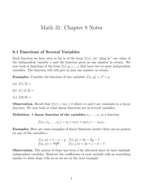
8.1 Functions of Several Variables
Each function we have seen so far is of the form f(x)...we “plug in” one value of
the independent variable x and the function gives us one number in return. We
now look at functions of the form f(x, y, z, ....) that have two or more independent
variables. The function will still give us just one number in return.
Examples. Consider the function of two variables f(x, y) = x 2 + y.
(a) f(1, 2) =
(b) f(−2, 3) =
(c) f(0, 0) =
Observation. Recall that f(x) = mx + b where m and b are constants is a linear
function. We now look at what linear functions are in several variables...
Definition. A linear function of the variables x 1 , . . . , x n is a function
f(x 1 , x 2 , . . . , x n ) = a 0 + a 1 x 1 + a 2 x 2 + · · · a n x n .
Examples. Here are some examples of linear functions (notice there are no powers
on any of the variables.)
f(x, y) = 1 − x − y f(x, y) = 3x − 2 7 y − 1
f(u, w) = u+4w
5
f(i, j, k) = 2i + j − k − 7
Observation. The notion of slope has been a bit obscured since we have multiple
independent variables. However the coefficients of each variable tells us something
similar to what slope tells us as we see in the next example:
1

Example. Let f(x, y) = 2 + 6x − 9y.
Example. Suppose the daily fixed cost for manufacturing cars and trucks at a plant
is $100 thousand . It costs $8 thousand to produce each truck and $6 thousand for
each car. Find the linear daily cost function C(x, y) for this plant.
Definition. If we add to a linear function a term of the form bx i x j with b ≠ 0 and
i ≠ j we get a second-order interaction equation.
Class Exercise. ($8.1 #12)
Example. The table gives the values of a function f(x, y).
(a) Find f(0, 1)
(b) f(2, 3) =
(c) Is f linear?
(d) Find an equation for f(x, y).
Class Exercise. (#8)
0 1 2 3
0 -1 0 1 2
1 3 4 5 6
2 7 8 9 10
3 11 12 13 14
2

8.2 Three-Dimensional Space and Graphs of Functions of
Two Variables
Graphs of functions of two variables f(x, y) lie in three-dimensional space (3-
space).
Plotting points in 3-space:
The familiar xy-plane has two axes, the x-axis and the y-axis. To form 3-space we
form another axis called the z-axis. A point in 3-space is specified by (x, y, z) and
we get to this point by going x units along the x-axis, y units along the y-axis, and
z units along the z-axis.
Example. Plot the points (1, 2, 3) and (−1, −2, 1).
Definition. The graph of a function of two variables z = f(x, y) is the set of
all points (x, y, f(x, y)) in 3-space. ( Of course, (x, y) must lie in the domain of f.)
Such a graph is often called a surface.
Example.
(a) Sketch the graph of z = 0 and z = 1 in 3-space.
(b) Sketch the graph of x = 0 and x = 1 in 3-space.
3

Example. Sketch the graph of the function z = f(x, y) = x 2 + y 2 .
Definition. If we have a surface z = f(x, y), and we fix a value for z, say z = c,
the set of all points satisfying c = f(x, y) is a level curve of the surface.
Graphs of Linear Functions: Planes The graphs of all linear functions are
planes. Looking at the graphs of z = 0 and z = 1 we get a clear picture of what
planes look like. For a general linear function the plane will be at some angle.
Example. Sketch z = f(x, y) = 1 − x − y.
(a) x-intercept (set y = z = 0):
(b) y-intercept (set x = z = 0):
(c) z-intercept (set x = y = 0):
Three points are enough to determine a plane. We can form a triangle from these
3 points. The plane of this triangle is the graph of f.
Alpha demonstration:
Class Exercise. ($8.2 #11-18)
4

8.3 Partial Derivatives
Recall. df
dx
is the derivative of f with respect to x. It tells us how fast is f changing
as x changes.
Definition. Let f(x, y, . . . ) be a function of several variables. The partial derivative
of f with respect to x is the derivative we get when we differentiate
f(x, y, . . . ) with respect to x while treating all other variables as constants. The
partial derivative of f with respect to x is denoted by ∂f
∂x
partial derivatives with respect to other variable, ∂f
∂y , ∂f
. We can similarly define
∂z , etc.
Notation.
• The symbol ∂f ∣
∂x (a,b)
means we evaluate the function ∂f
∂x
at the point (a, b).
• ∂f
∂x
and
∂f
∂y are also denoted by f x and f y .
Examples. Let f(x, y) = x 2 − 4xy.
(a) ∂f
∂x =
(b) ∂f ∣
(1,1)
=
∂x
(c) ∂f
∂y =
(d) If C(x, y) is a cost function, ∂C
∂x
and
∂C
∂y
are the marginal cost functions.
Class Exercise. ($8.3 #46) Interpret your answer.
Interpretation of Partial Derivatives and Marginal Costs:
The partial derivative ∂C ∣
∂x (a,b)
is the approx. cost of the (a + 1) st “x” item, and
∣
(a,b)
is the approx. cost of the (b + 1) st “y” item.
∂C
∂y
5

Geometric Interpretation of Partial Derivatives:
∂f ∣
∂x (a,b)
is the slope of the tangent line to the surface z = f(x, y) in the vertical
plane y = b, and ∂f ∣
∂y (a,b)
is the slope of the tangent line to the surface z = f(x, y)
in the vertical plane x = a.
Second-Order Partial Derivatives: These will be helpful when we study how
to maximize and minimize functions of two variables.
• f xx = (f x ) x = ∂2 f
∂x 2
= ∂
∂x (∂f ∂x )
• f yy = (f y ) y = ∂2 f
∂y 2
= ∂ ∂y (∂f ∂y )
• f xy = (f x ) y = ∂2 f
∂y∂x = ∂ ∂y (∂f ∂x )
• f yx = (f y ) x = ∂2 f
∂x∂y = ∂
∂x (∂f ∂y )
Fact. Amazingly, we always have f xy = f yx !
Class Exercises. As you compute these, verify that f xy = f yx .
(a) ($8.3 #24)
(b) ($8.3 #26)
6

8.4 Maxima and Minima (2 Lectures )
Day 1 : Types of Max/Min and Critical Points
Definition. Let f(x, y, . . . ) be a function of several variables.
• f has a relative maximum at the point (r, s, . . . ) if the value f(r, s, . . . ) is
bigger than all other values in the immediate vicinity.
• f has a relative minimum at the point (r, s, . . . ) if the value f(r, s, . . . ) is
smaller than all other values in the immediate vicinity.
• f has a absolute maximum at the point (r, s, . . . ) if the value f(r, s, . . . )
is the largest value of the function over its entire domain.
• f has a absolute minimum at the point (r, s, . . . ) if the value f(r, s, . . . ) is
the smallest value of the function over its entire domain.
Definition. Relative maxima and relative minima are called the relative extrema
of f
Observation. Absolute maxima and absolute minima are special kinds of relative
extrema.
All the above definitions have analogous notions in the single variable case. The
next notion is not analogous to anything in the single variable case:
Definition. Let f(x, y) be a function of two variables. f has a saddle point at
(r, s) if f has a relative maximum along some slice through the point, and a relative
minimum along some other slice through the point.
Candidates for Extrema: Critical Points
Definition. Points in the domain of f where all partial derivatives are zero are
critical points of f.
Fact. Critical points of f are the only candidates for relative extrema and saddle
points of f in the interior of the domain of f.
7

Warning. A critical point is not necessarily an extrema or saddle point! Further
checks are needed to determine whether it is or not.
Next lecture we will learn a test to determine if a critical point gives an extrema
or not.
Example. ($8.4 #14) Find all critical points of the function g(x, y) = x 2 + x +
y 2 − y − 1.
Class Exercise. ($8.4 #28) Find all critical points of the function g(x, y) = x 3 +
y 3 + 3
xy . 8

8.4 Maxima and Minima - Day 2
GOAL: Classify Critical Points
Definition. Let f be a function of two variables and (a, b) be a critical point. The
quantity
H = H(a, b) = f xx (a, b)f yy (a, b) − [f xy (a, b)] 2
is called the Hessian at the point (a, b).
Fact. (Second Derivative Test) Let f be a function of two variables and (a, b)
be a critical point.
1. If H(a, b) > 0, then,
• f has a relative min at (a, b) if f xx (a, b) > 0
• f has a relative max at (a, b) if f xx (a, b) < 0,
2. If H(a, b) < 0,
• f has a saddle point at (a, b).
3. If H(a, b) = 0,
• The test is inconclusive. A table or graph can be used to decide what
kind of extrema exist at (a, b).
Example. ($8.4 #12) Find and classify all the critical points of f(x, y) = 4−(x 2 +
y 2 ).
9

Class Exercise. ($8.4 #20) Find and classify all the critical points of t(x, y) =
x 3 − 3xy + y 3 .
Example. Find and classify all the critical points of f(x, y) = y 2 .
Example. Find and classify all the critical points of f(x, y) = x 3 .
10

8.5 Constrained Maxima and Minima
We have seen how to find extrema of functions over their entire domains.
GOAL: Find Max and Mins of a function f subject to constraints (over
restricted domain)
Example. If you want to make a closed box with square bases that holds 125 cm 3 ,
what box dimensions produce a box requiring the least material?
Example. Find the maximum value of the function f(x, y, z) = 4 − (x 2 + y 2 + z 2 )
subject to the constraint (a) z = 2x and (b) z = 1.
Idea: Solve the constraint for one of the variables and substitute. Then
maximize the resulting function of two variables.
Example. If you want to make an open-top rectangular box that will hold 4 cm 3 ,
what box dimensions produce a box requiring the least material?
Class Exercise. ($8.5 #6)
11

Example. ($5.2 #20)
Preview of Next Lecture: Sometimes it is too hard or impossible to eliminate
one of the variables. For example, imagine if the constraint equation was x 2 +y 2 = 1
or (zxy) 3 = x 7 + y 8 − z 9 . In such cases we can use the method of Lagrange Multipliers.
We will discuss this method next lecture. Even if it is possible to solve
for one of the variables, Lagrange multipliers always provides an alternative way
to find extrema and can sometimes be quicker.
Distance functions: The distance between two point P (x 1 , y 1 ) and Q(x 2 , y 2 ) in
the xy−plane is
d = √ (x 2 − x 1 ) 2 + (y 2 − y 1 ) 2
.
For two points in 3-space P (x 1 , y 1 , z 1 ) and Q(x 2 , y 2 , z 2 ) the distance between
them is
d = √ (x 2 − x 1 ) 2 + (y 2 − y 1 ) 2 + (z 2 − z 1 ) 2
.
Example. Find the distance between the points (3, −2) and (−1, 1).
Example. Find the distance between the points (1, 1, 1) and (−1, 1, 2).
Fact. The equation for a circle of radius r with center at the origin is
x 2 + y 2 = r 2 .
Question. What geometric shape in 3-space is given by the solutions to the equation
x 2 + y 2 + z 2 = r 2 ?
12

Constrained Maxima and Minima - Day 2
Lagrange Multipliers
Fact. Locating Relative Extrema with Lagrange Multipliers
The candidates for relative extrema of f(x, y, . . . ) subject to the constraint g(x, y, . . . ) =
0 are the solutions to equations
f x = λg x
f y = λg y
· · ·
g = 0
The constant λ is called a Lagrange multiplier.
Observation. The value of the Lagrange multiplier λ does not matter; hence, it
is usually a good idea to try to eliminate it from the system of equations as early
as possible.
Example. Maximize f(x, y) = xy subject to the constraint x 2 + y 2 = 2.
Warning. If we assume extrema exist there is no problem with just evaluating at
critical points and comparing, but be aware that we are making an assumption
here.
Class Exercise. ($8.5 #12) Minimize f(x, y) = x 2 + y 2 subject to constraint
xy 2 = 16.
13

Example. ($8.5 #22)
Example. ($8.5 #28) Find point on plane 2x − 2y − z + 1 = 0 closest to (1, 1, 0).
14