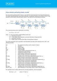
Waterman, D., Broere, W., 2004, Application of the SSC model - Plaxis

The second possibility to assign a correct OCR value in Plaxis is to leave the OCR equal
to 1 in the initial conditions and start the calculation with a plastic nil step. For this
phase set the time interval equal to ∆t. Plaxis will now calculate the stress state due
the creep over that period, which results in a certain OCR. In the second phase of the
calculation the settlements due to the simulation of the creep history must be discarded
using the “reset displacements to zero” option in Plaxis Calculations.
Generally, if ∆t is large the exact value becomes less important, as the OCR depends
on natural logarithm of time. It makes a large difference whether soil has been in place
for 10 days or 1 year, but there will be relatively little additional creep between 100
years or 200 years.
When generating the initial stresses using the K 0 -procedure, the influence of the OCR
warrants some extra attention. The initial vertical preconsolidation stress at a certain
depth is calculated, as might be expected, from the effective weight of the soil on top
multiplied by the OCR value that has been entered (σ c = OCR . σ' y ). When a plot of the
OCR values obtained in this way is inspected, it can be noticed that the reported OCR
values differ slightly from the enter value. The reason for this is that the OCR value
Plaxis Output reports is calculated using the stress measure p eq , defined as
This stress measure is used internally by Plaxis to define OCR from p p = OCR . p eq . The
reason for this is that the regular definition of OCR (σ c = OCR . σ' y ) is not always
meaningful in complex 3D loading situations. And although it would be preferable to
report OCRs using the same definition as used in the initial conditions, unfortunately it
is not possible to derive Cartesian stresses from p eq in case the cohesion is nonzero.
In order to illustrate this a simple example is given. Define in Plaxis V8 a square of 1x1m
with standard boundary conditions and a distributed load on top.
Define a material data set using the Soft Soil Creep model and the material type set to
drained. Other material parameters are given in table 1. Normally one would use
undrained material behaviour but to more clearly illustrate creep only drained behaviour
is selected here.
Parameter Name Value Unit
Material model Model Soft Soil Creep -
Type of material behaviour Type Drained -
Unit weight of soil above phreatic level γ unsat 17.0 kN/m 3
Unit weight of soil below phreatic level γ sat 17.0 kN/m 3
Modified compression modulus λ* 0.025 -
Modified swelling modulus κ* 0.010 -
Modified creep modulus µ* 0.001 -
Cohesion (constant) c ref 1.0 kN/m 2
Friction angle φ 28.0 º
Dilatancy angle ψ 0.0 º
Table 1: Material parameters
For this case the sample is assumed dry and for initial stresses generation the default
values for K 0 and OCR are used. The calculation consists of 5 phases:
1. A load of -100 kPa is applied at the top with time interval zero.
2. A staged construction phase with a time interval of 100 days. Use the “reset displacements
to zero” option.
3. Starting from the initial phase once more add a staged construction phase with a
time interval of 36500 days (100 years).
4. A load of -100 kPa is applied at the top with time interval zero.
5. A staged construction phase with a time interval of 100 days. Use the “reset displacements
to zero” option.
Start the calculation and ignore the warning about calculation phases with zero time
interval.
Figure 2 shows a graph of the displacements vs. time for a node in the sample. The
additional resting time of phase 3 increased the OCR from 1 to approximately 2.4
resulting in a stiffer behaviour of the sample as can be seen from the figure.
0,000
-0,005
Uy (m)
-0,010
-0,015
-0,020
-0,025
-0,030
-0,035
loading after 100 years
-0,040
-0,045
immediate loading
-0,050
0 20 40 60 80 100 120
Time (days)
Figure 1: Geometry used in this example.
Figure 2: Time - settlement curve.
15