FE-Analysis of piled and piled raft foundations - Plaxis

FE-Analysis of piled and piled raft foundationsJean-Sébastien LEBEAUApril - August 2008

AcknowledgementsFirst of all I would like to express my gratefulness to Professor Helmut F. Schweiger for giving methe opportunity to work on geotechnical issues at the Institute for Soil Mechanics and FoundationEngineering of Graz University of Technology.This paper was made possible by the great contribution of my supervisor Dipl.-Ing Franz Tschuchnigg.I am indebted to him for his friendly supervision and guidance throughout the period of mytraineeship. I deeply thank him because he conveyed me a better understanding of nite elementmodeling and analyses.I also would like to thank my French professor, Yvon Riou for getting me in touch with the Institute.Finally, I would like to express my appreciation to all the people I met here who made my ve monthsstay in Austria very enjoyable.2

Contents1 Introduction 62 Preliminary studies 72.1 Single pile . . . . . . . . . . . . . . . . . . . . . . . . . . . . . . . . . . . . . . . . . . 72.1.1 Presentation of calculations . . . . . . . . . . . . . . . . . . . . . . . . . . . . 72.1.1.1 Geometry . . . . . . . . . . . . . . . . . . . . . . . . . . . . . . . . . 72.1.1.2 Boundaries conditions . . . . . . . . . . . . . . . . . . . . . . . . . . 82.1.1.3 Material properties . . . . . . . . . . . . . . . . . . . . . . . . . . . . 82.1.1.4 Meshes . . . . . . . . . . . . . . . . . . . . . . . . . . . . . . . . . . 92.1.1.5 Load control and calculation steps . . . . . . . . . . . . . . . . . . . 102.1.2 Results . . . . . . . . . . . . . . . . . . . . . . . . . . . . . . . . . . . . . . . 102.1.2.1 Mesh dependency . . . . . . . . . . . . . . . . . . . . . . . . . . . . 112.1.2.2 Comparison between distributed loads and prescribed displacement 142.1.2.3 Inuence of the interface coecient R inter . . . . . . . . . . . . . . . 162.1.2.4 Inuence of the dilatancy . . . . . . . . . . . . . . . . . . . . . . . . 172.2 Pile-raft . . . . . . . . . . . . . . . . . . . . . . . . . . . . . . . . . . . . . . . . . . . 182.2.1 Presentation of calculations . . . . . . . . . . . . . . . . . . . . . . . . . . . . 182.2.1.1 Geometry . . . . . . . . . . . . . . . . . . . . . . . . . . . . . . . . . 182.2.1.2 Boundaries conditions . . . . . . . . . . . . . . . . . . . . . . . . . . 192.2.1.3 Materials properties . . . . . . . . . . . . . . . . . . . . . . . . . . . 192.2.1.4 Meshes . . . . . . . . . . . . . . . . . . . . . . . . . . . . . . . . . . 192.2.1.5 Load control and calculation steps . . . . . . . . . . . . . . . . . . . 202.2.2 Results . . . . . . . . . . . . . . . . . . . . . . . . . . . . . . . . . . . . . . . 203

CONTENTSCONTENTS2.2.2.1 Mesh dependency . . . . . . . . . . . . . . . . . . . . . . . . . . . . 202.2.2.2 Inuence of the interface coecient R inter . . . . . . . . . . . . . . . 212.2.2.3 Inuence of the dilatancy . . . . . . . . . . . . . . . . . . . . . . . . 223 Analysis of 2D models 243.1 Single-pile . . . . . . . . . . . . . . . . . . . . . . . . . . . . . . . . . . . . . . . . . . 243.2 Pile-Raft . . . . . . . . . . . . . . . . . . . . . . . . . . . . . . . . . . . . . . . . . . . 263.2.1 Load-displacement curve . . . . . . . . . . . . . . . . . . . . . . . . . . . . . . 293.2.2 Variations of Skin friction and Normal Stresses along the pile . . . . . . . . . 293.2.3 Analysis of the α Kpp factor . . . . . . . . . . . . . . . . . . . . . . . . . . . . 363.2.3.1 Denition of α Kpp . . . . . . . . . . . . . . . . . . . . . . . . . . . . 363.2.3.2 Methodology to calculate α Kpp . . . . . . . . . . . . . . . . . . . . . 373.2.3.3 Comparison and evolution of α Kpp for dierent geometries: . . . . . 393.2.3.4 Evolution of α Kpp for dierent materials and dilatancy . . . . . . . . 413.2.3.5 Evolution of α Kpp for dierent values of R inter . . . . . . . . . . . . 423.2.4 Eciency of a piled-raft foundation in comparison with a raft foundation . . 443.2.5 Analysis of the pile behavior . . . . . . . . . . . . . . . . . . . . . . . . . . . . 453.2.5.1 Base resistance . . . . . . . . . . . . . . . . . . . . . . . . . . . . . . 453.2.5.2 Skin resistance . . . . . . . . . . . . . . . . . . . . . . . . . . . . . . 463.2.5.3 Conclusions . . . . . . . . . . . . . . . . . . . . . . . . . . . . . . . . 474 Preliminary studies of 3D models 494.1 Volume pile . . . . . . . . . . . . . . . . . . . . . . . . . . . . . . . . . . . . . . . . . 504.1.1 Finite element models . . . . . . . . . . . . . . . . . . . . . . . . . . . . . . . 504.1.2 Results . . . . . . . . . . . . . . . . . . . . . . . . . . . . . . . . . . . . . . . 524.1.2.1 Load-displacement curves . . . . . . . . . . . . . . . . . . . . . . . . 524.1.2.2 Variations of skin friction . . . . . . . . . . . . . . . . . . . . . . . . 544.1.2.3 Some remarks about parameters . . . . . . . . . . . . . . . . . . . . 584.2 Embedded pile . . . . . . . . . . . . . . . . . . . . . . . . . . . . . . . . . . . . . . . 604.2.1 Embedded pile-raft . . . . . . . . . . . . . . . . . . . . . . . . . . . . . . . . . 604.2.1.1 Finite element models . . . . . . . . . . . . . . . . . . . . . . . . . . 614

CONTENTSCONTENTS4.2.1.2 Embedded pile with linear skin friction distribution . . . . . . . . 634.2.1.3 Embedded pile with multilinear skin friction distribution . . . . . 694.2.1.4 Embedded pile with layer dependent skin friction distribution . 734.2.1.5 Comparison of the three options: Linear, multilinear and layer dependent. . . . . . . . . . . . . . . . . . . . . . . . . . . . . . . . . . 775 Group eect 825.1 Presentation of calculations . . . . . . . . . . . . . . . . . . . . . . . . . . . . . . . . 825.1.1 Geometry . . . . . . . . . . . . . . . . . . . . . . . . . . . . . . . . . . . . . . 835.1.2 Finite element model . . . . . . . . . . . . . . . . . . . . . . . . . . . . . . . . 865.2 Results . . . . . . . . . . . . . . . . . . . . . . . . . . . . . . . . . . . . . . . . . . . . 865.2.1 Vocabulary details . . . . . . . . . . . . . . . . . . . . . . . . . . . . . . . . . 865.2.2 Load-displacement curves . . . . . . . . . . . . . . . . . . . . . . . . . . . . . 875.2.3 Displacement proles . . . . . . . . . . . . . . . . . . . . . . . . . . . . . . . . 895.2.4 More precise analysis of group 5 . . . . . . . . . . . . . . . . . . . . . . . . . 925.2.5 Conclusion . . . . . . . . . . . . . . . . . . . . . . . . . . . . . . . . . . . . . 976 Conclusion 985

Chapter 1IntroductionIn traditional foundation design, it is customary to consider rst the use of shallow foundation suchas a raft (possibly after some ground-improvement methodology performed). If it is not adequate,deep foundation such as a fully piled foundation is used instead. In the last few decade, an alternativesolution has been designed: piled raft foundation. Unlike the conventional piled foundation design inwhich the piles are designed to carry the majority of the load, the design of a piled raft foundationallows the load to be shared between the raft and piles and it is necessary to take the complexsoil-struture interaction eects into account.The concept of piled raft foundation was rstly proposed by Davis and Poulos in 1972 and is nowused extensively in Europe, particularly for supporting the load of high buildings or towers. Thefavorable application of piled raft occurs when the raft has adequate loading capacities, but thesettlement or dierential settlement exceed allowable values. In this case, the primary purpose ofthe pile is to act as settlement reducer.The aim of this paper is to describe a nite element analysis of deep foundations: piled and mainlypiled raft foundations. A basic parametric study is rstly presented to determine the inuence ofmesh discretisation, of materials - loose or dense sand -, of dilatancy and interface elements. Thenthe behavior of piled raft foundations is analysed in more details using partial axisymmetric modelsof one pile-raft.We continue by preparing a more sophisticated 3D study to take into account the complex pilepileinteraction which occured when the pile spacing is small. So the possibilies of employing theembedded pile concept as implemented into Plaxis 3D foundations is investigated. Finally, someclues about the group eect are indicated.6

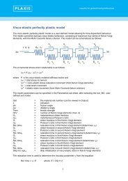
2.1. SINGLE PILE CHAPTER 2. PRELIMINARY STUDIES2.1.1.2 Boundaries conditionsWe used the standard xities PLAXIS tool to dene the boundaries conditions. Thus these boundariesconditions are generated according to the following rules:ˆVertical geometry lines for which the x-coordinate is equal to the lowest or highest x-coordinatein the model obtain a horizontal xity (u x = 0).ˆHorizontal geometry lines for which the y-coordinate is equal to the lowest y-coordinate in themodel obtain a full xity (u x = u y = 0).Figure 2.1: Global geometry of the axisymmetric model of the single pile2.1.1.3 Material propertiesThe constitutive model used for the soil - sand - is the Hardening soil model. The main advantageof this constitutive law is its ability to consider the stress path and its eect on the soil stiness andits behavior. We used two dierent types of sand: one loose and the other dense. We also variedthe dilatancy value.8

2.1. SINGLE PILE CHAPTER 2. PRELIMINARY STUDIESFor the concrete pile, a linear elastic material set was applied.The parameters of all this materials are summarized in the following table:Parameter Symbol Loose sand Dense sand Concrete (pile) UnitMaterial model Model Hardening Soil Hardening Soil Linear Elastic -Unsaturated weigth γ unsat 17 19 25 kN/m 3Saturated weigth γ sat 20 21 25 kN/m 3Permeability k 1 1 0 m/dayE ref50 20 000 60 000 kN/m 3StinessEur ref 1E5 1,8E5 kN/m 3Power m 0,65 0,55Poisson ratio ν ur 0,2 0,2 0,2 -Dilatancy y 2/0 8/0 °Friction angle f 32 38 °Cohesion c ref 0,1 0,1 kN/m 2Lateral pressure coe. K 0 1-sinf 1-sinf -Failure ratio Rf 0,9 0,9 -E refoed20 000 60 000 3E7 kN/m 3Table 2.1: Materials parameters2.1.1.4 MeshesTo study the mesh dependency 3 analyses were performed: one with a coarse, one with a mediumand one with a very ne mesh. For each one we considered 6 models varying the interface elements.Thus we played around the R inter coecient 2 from 0,1 to 1.2 This factor relates the interface strength (wall friction and adhesion) to the soil strength (friction angle andcohesion)9

2.1. SINGLE PILE CHAPTER 2. PRELIMINARY STUDIESFigure 2.2: A very ne mesh for calculations with interface elementsCoarse Medium Very neNumber of elements 611 1848 4365Number of nodes 5215 15 389 36 019Elements15-nodeTable 2.2: Information on the generated meshes2.1.1.5 Load control and calculation stepsTo assign a load at the top of the pile we considered two approaches: one with prescribed displacement,one with distributed loads.With prescribed displacement we impose a certain displacement at the top of the pile whereas withdistributed loads we impose a force; results should be the same.2.1.2 ResultsRemark: All the following curves are plotted for the node point located at the top right side ofthe pile.10

2.1. SINGLE PILE CHAPTER 2. PRELIMINARY STUDIESFigure 2.3: Node point selected for load-displacement curves2.1.2.1 Mesh dependencyBy analysing all the calculations made, we can conclude that for each material - loose or dense sand- the curves have the same shapes for calculations performed with coarse, medium andvery ne mesh. Nevertheless, we can observe that with ner meshes, we have unphysical prematuresoil body collapsing. The following gure illustrates this conclusion with some examples.11

2.1. SINGLE PILE CHAPTER 2. PRELIMINARY STUDIESFigure 2.4: Mesh dependency for the loose sand - ψ=2° - and dierent values for R interles : Geo2Load_Mesh 1/2/3_Rinter0,1/0,7/1_Psi2_HS.plxTo avoid this premature failure we decided to restart the medium and very ne calculations switchingo the arc length control procedure. But we now observed convergence problems with more or lessimportant oscillations.These oscillations occurred for important displacements (from 20 cm) whatever the material, meshor R inter value. However, the global shape of the load-displacement curve seems to stay realisticeven if there are these stairs.12

2.1. SINGLE PILE CHAPTER 2. PRELIMINARY STUDIESFigure 2.5: Mesh dependency for the loose sand - ψ=2° - and dierent values for R interles : Geo2Load_Mesh 2_Loose_Rinter0,1/0,7_Psi2_HS(_alc=OFF).plxFigure 2.6: Inuence of arc length control for the loose sand - ψ=2° - and R inter =0,7/0,1parameters: mesh1= coarse, arc length=ON; mesh2= medium, arc length=OFF; mesh3= Very ne, arclength=OFF;13

2.1. SINGLE PILE CHAPTER 2. PRELIMINARY STUDIESThe gure 2.6 enables us to conrm that the mesh dependency is negligible for this model.2.1.2.2 Comparison between distributed loads and prescribed displacementThe previous paragraph was based on les with the load approach. We did the same calculations withthe displacement approach. By comparing these two approaches we can conclude that the shapeof the load-settlement curves is exactly the same in each case. Moreover, there are lessoscillations with prescribed displacement than with distributed loads. There are no stairs'' evenwith an important displacement. So because it limits this problem of big oscillations, prescribeddisplacement seems to be better to study a single pile. The following picture illustratesthese conclusions.Figure 2.7: Distributed loads and prescribed displacement, comparison for the loose sand - ψ=0°- and R inter =0,1/0,4/0,7les : Geo2Disp/Load_Mesh 2_Rinter0,1/0,4/0,7_Psi0_HS(_alc=OFF).plx14

2.1. SINGLE PILE CHAPTER 2. PRELIMINARY STUDIESRemark: The gure 2.7 shows us the settlement with the load [kN] whereas in the previous sectionwe plotted the settlement with the distributed load [kN/m 2 ]. To compare the two approaches we haveto:ˆˆDistributed load: Multiply the distributed load [kN/m 2 ] by the area of the pile to get the totalforce (R tot ) [kN].Prescribed displacement: Read out the force value in Plaxis output [kN/rad] and multiply itby 2 π to get the total force (R tot ) [kN]Now we can try to interpret the stairs of the load approach by comparing with the same calculationsdone with the prescribed displacements.Figure 2.8: Comparison Displ and Load approaches for the loose sand ψ=0°medium mesh- No interface les : Geo2Disp/Load_Mesh 2_Loose_RinterNo_Psi=0_HS(_alc=OFF).plx15

2.1. SINGLE PILE CHAPTER 2. PRELIMINARY STUDIESFigure 2.9: Comparison Displ and Load approaches for the loose sand ψ=0° - R=1 medium meshles : Geo2Disp/Load_Loose_Mesh 2_Rinter1_Psi=0_HS(_alc=OFF).plxAs we can see on gures 2.8 and 2.9, it is impossible to deduce correctly the normal shape from thedistributed load curves by interpreting the oscillations. Sometimes, the prescribed displacementcurve is under the distributed load one, sometimes it is in the middle. So we have to interpretwith caution the shape of the stairs part of the distributed load curves.2.1.2.3 Inuence of the interface coecient R interWe varied the way to model the pile to sand interface by changing the R inter value and doing a modelwithout interface. We also performed one calculation by drawing an interface in Plaxis input andunselected it in Plaxis calculation.We can conclude that the choice of the value for R inter is not negligible when you modela single pile. As we can see in the table, for the same load, the settlements increase by more than40 % between R=0,4 and 0,1, 80% between R=0,7 and 0,4 and 600 % between R=1 and 0,7 forloose sand.Load=2000 kNSettlement [cm]R inter =0,1 22,5R inter =0,4 15,7R inter =0,7 8,6R inter =1 1,2Table 2.3: Settlements of the single pile for loose sand, ψ=2° and R tot =2000 kN16

2.1. SINGLE PILE CHAPTER 2. PRELIMINARY STUDIESAs we could expect the load-displacement curves have almost the same shape for models with R=1and without interface. We also noticed that unselecting the interface lead to false results withpremature failure (see red following curve) or an unrealistic behavior. So the interface drawn inthe Plaxis input must be selected in the calculations steps. The following curves sum up all theseconclusions.Figure 2.10: Load-settlement curves for Loose sand, ψ=2° and coarse meshles : Geo2Load_Mesh1_Loose_Rinter0,1/0,4/0,7/1/Unselected/No_Psi=2_HS.plx2.1.2.4 Inuence of the dilatancyWe tested two values of dilatancy ψ for both materials: (ϕ − 30) and 0°. As expected, we have lessdisplacement with a high ψ value than without dilatancy.17

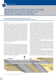
2.2. PILE-RAFT CHAPTER 2. PRELIMINARY STUDIESFigure 2.11: Inuence of dilatancy for dense sand, mesh mediumles : Geo2Load_Mesh2_Dense_Rinter0,4/0,7_Psi8/0_HS_ALCo.plx2.2 Pile-raft2.2.1 Presentation of calculations2.2.1.1 GeometryWe performed the same calculations as we have done with the single pile model using an axisymmetricmodel of a pile-raft foundation.As we did for the single pile, the pile has been modeled with a length of 15 m and a diameter of0,8 m at the axis of symmetry. We added a slab in concrete with a thickness of 0,5 m. The soil isalso modeled as a single layer of sand with the same properties as the single pile. The ground wateris located at 40 m below the soil surface. In this way we did not take into account the waterinuence. Along the length of the pile an interface has been modeled. We extended this interfaceto 0,5 m below the pile inside the soil body to prevent stress oscillation in this sti corner area.18

2.2. PILE-RAFT CHAPTER 2. PRELIMINARY STUDIES2.2.1.2 Boundaries conditionsWe also used for this study the standard xities PLAXIS tool (see 2.1.1.2).2.2.1.3 Materials propertiesThe parameters of all the materials are recalled in the following table:Parameter Symbol Loose sand Dense sand Concrete UnitMaterial model Model Hardening Soil Hardening Soil Linear Elastic -Unsaturated weigth γ unsat 17 19 25 kN/m 3Saturated weigth γ sat 20 21 25 kN/m 3Permeability k 1 1 0 m/dayE ref50 20 000 60 000 kN/m 3StinessEur ref 1E5 1,8E5 kN/m 3Power m 0,65 0,55Poisson ratio ν ur 0,2 0,2 0,2 -Dilatancy y 2/0 8/0 °Friction angle f 32 38 °Cohesion c ref 0,1 0,1 kN/m 2Lateral pressure coe. K 0 1-sinf 1-sinf -Failure ratio Rf 0,9 0,9 -E refoed20 000 60 000 3E7 kN/m 3Table 2.4: Materials parameters2.2.1.4 MeshesTo study the mesh dependency 3 analysis were also performed: one with a coarse, one with a mediumand one with a very ne mesh. For each one we considered 6 models varying the interface elements.Thus we varied the R inter coecient from 0,1 to 1. We also performed one batch of calculation with6-nodes instead of 15 nodes.Coarse Medium Very ne CoarseNumber of elements 459 1417 3012 903Number of nodes 4246 12 578 25 708 2211Elements 15-node 6-nodeTable 2.5: Information on the generated meshes19

2.2. PILE-RAFT CHAPTER 2. PRELIMINARY STUDIES2.2.1.5 Load control and calculation stepsTo assign a load at the top of the slab we considered in this case only a distributed loadFigure 2.12: Details about a pile-raft geometry with the axisymmetric model, Very ne mesh2.2.2 ResultsRemark: All the following curves are plotted for the node point A, situated at the top right sideof the pile, under the slab (see gure 2.12).2.2.2.1 Mesh dependencyBy analysing all the calculations made, we can conclude that for each material - loose or densesand - the curves have exactly the same shapes for calculations performed with coarse,medium and very ne mesh.20

2.2. PILE-RAFT CHAPTER 2. PRELIMINARY STUDIESFigure 2.13: Example, Mesh dependency for the pile raft model with loose sand, ψ=2°, R inter =0,7les : Geo1_Mesh1/2/3_loose_Rinter0,7_Psi2_HS.plx2.2.2.2 Inuence of the interface coecient R interWe varied the way to model the pile to sand interface by changing the R inter value and doing a modelwithout interface.As we can see in the table and on the following curve the way you model the interface has anegligible inuence on the settlements.Sand Mesh ψ R inter =0,4 R inter =0,7 R inter =1Loose Coarse 2° -34,3 cm -33,0 cm -32,4 cmDense Coarse 8° -13,6 cm -13,2 cm -13,0 cmTable 2.6: Settlements with dierent values of R inter for load=1000 kN/m 221

2.2. PILE-RAFT CHAPTER 2. PRELIMINARY STUDIESTable 2.7: Load-settlement curves for Loose sand, ψ=2° and coarse meshles : Geo1_Mesh1_loose_Rinter0,1/0,4/0,7/1/NO_Psi2_HS.plx2.2.2.3 Inuence of the dilatancyWe tested two values of dilatancy (ψ) for both materials: 2° and 0° for the loose sand, 8° and 0° forthe dense sand. We can conclude that the inuence of the dilatancy is negligible for thismodel even for the dense sand.Sand Mesh ψ R inter =0,4 R inter =0,7 R inter =1Loose Coarse 2° -34,3 cm -33,0 cm -32,4 cmLoose Coarse 0° -34,4 cm -33,0 cm -32,4 cmDense Coarse 8° -13,6 -13,2 -13,0Dense Coarse 0° -13,7 -13,2 -13,1Table 2.8: Settlements with dierent values of R inter for load=1000 kN/m 222

2.2. PILE-RAFT CHAPTER 2. PRELIMINARY STUDIESFigure 2.14: Inuence of dilatancy for dense sand, mesh coarseles : Geo1_Mesh1_dense_Rinter0,4/0,7_Psi8/0_HS.plx23

Chapter 3Analysis of 2D models- Behavior of a pile and a pile-raft -In chapter 2 we made conclusions about how to dene eciently and correctly an axisymmetricmodel of a single pile and a pile-raft. Now we present other calculations performed by taking thesepreliminary practical conclusions into account.In design of piled rafts, design engineers have to understand the mechanism of load transfer fromthe raft to the piles and to the soil. It requires to take complex interactions into account such as:pile-soil interaction, raft-soil interaction, pile-raft interaction and pile-pile interaction.The aim of this chapter is to have a better understanding of the pile and raft behavior and to checkthe ability of the software to model such complex interactions. In this part, we only modeled a singlepile with a raft so we did not take into account the pile-pile interaction.3.1 Single-pileIn the previous calculations we simulated an axial load test on a bored pile. We get the followingload-displacement curve:24

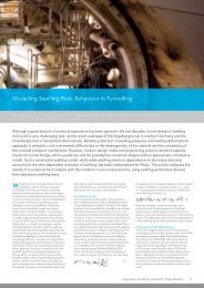
3.1. SINGLE-PILE CHAPTER 3. ANALYSIS OF 2D MODELSFigure 3.1: Axial load curve for a single-pilele : Geo2Disp_Mesh2_loose_R=0,7_Psi2_HS.plxNow we observe the mobilisation of the skin friction (q s ) with dierent loads.Figure 3.2: Evolution of the Skin friction with the load (Rtot)le : Geo2Disp_Mesh2_loose_R=0,7_Psi2_HS.plx25

3.2. PILE-RAFT CHAPTER 3. ANALYSIS OF 2D MODELSs = 1cm s = 8cm s = 15cmR b [kN] 140 906 1380R s [kN] 1050 1044 1040R sR b7,5 1,15 0,75Table 3.1: Evolution of the skin and base resistance with settlementsle : Geo2Disp_Mesh2_loose_R=0,7_Psi2_HS.plxThat shows that the maximum skin friction is already reacted when 1,0 cm settlements occur (seegure 3.1). Further, the skin resistance stays the same.3.2 Pile-RaftKey questions that arise in the design of piled rafts concern the relative proportion of load carriedby raft and piles. It depends on the geometric parameters of the pile and of the raft.We performed four new models based on the rst geometry described in chapter 2 to interpret theraft and pile inuence 1 .Figure 3.3: Some geometric parameters1 The Pile-Raft I is the geometry described in details in the chapter 226

3.2. PILE-RAFT CHAPTER 3. ANALYSIS OF 2D MODELSParamater Symbol Pile-Raft I Pile-Raft IIDiameter of the pile d pile 0,8 m 0,8 mLength of the pile L pile 15 m 15 mWidth of the raft L raft 2 m 5 mDepth of the model H model 40 m 40 mThickness of the slab t raft 0,5 m 0,5 mL raftd pile2,5 6,25Table 3.2: Parameters of the rst set of calculationsFigure 3.4: Details of Pile-Raft I and II27

3.2. PILE-RAFT CHAPTER 3. ANALYSIS OF 2D MODELSParamater Symbol Pile-Raft V Pile-Raft III Pile-Raft IVDiameter of the pile d pile 1,5 m 1,5 m 1,5 mLength of the pile L pile 30 m 30 m 30 mWidth of the raft L raft 4,5 m 9 m 18 mDepth of the model H model 60 m 60 m 60 mThickness of the slab t raft 1 m 1 m 1 mL raftd pile3 6 12Table 3.3: Parameters of the second set of calculationsFigure 3.5: Details of Pile-Raft V, III and IVWe tested all these geometries with the materials loose and dense sand 2 , with and without dilatancyand varying the value of R inter . The outcome was that the inuence of dilatancy and ofR inter is very limited. We also performed these calculations with 3 dierent meshes to conrmthat there is no mesh dependency. We tryed to have next the pile the same mesh coarseness in2 See table n°2.428

3.2. PILE-RAFT CHAPTER 3. ANALYSIS OF 2D MODELSeach model in order to compare precisely the dierent models. The load is a distributed load appliedon the slab and the boundaries conditions are those described in chapter 2. In this study we didnot take into account the ground water.Remark: As we did in chapter 2, all the load-displacement curves are plotted for the node pointA, situated at the top right side of the pile, under the slab (see gure 2.12).3.2.1 Load-displacement curveAs we see on the following gure, the load-displacement curve for a pile-raft and a single pile iscompletely dierent.Figure 3.6: Load settlement curve for pile and pile-raft foundationles : Geo1/1Bis/2load_Mesh1_loose_R=0,7_Psi2_HS.plx3.2.2 Variations of Skin friction and Normal Stresses along the pileFor each model we plotted the skin friction and the normal stresses along the pile. This proceduregave us the possibility to illustrate how the load transfer works when the load increases. All thefollowing curves concern dense sand with ψ=8° and R inter = 0, 7 3 .3 According to Plaxis manual this Rinter value is the most common to model standard situations29

3.2. PILE-RAFT CHAPTER 3. ANALYSIS OF 2D MODELSRemark: All these gures are plotted by selecting the interface in the Plaxis output. In order toget something comparable from one model to an other, we subtracted the rst phase with the pileactivationfor each load steps plotted. Thus the Skin friction or Normal Stresses that we presenthere are only due to the load and the weight of slab.Figure 3.7: Evolution of the skin friction with the load for the Pile-raft I ( d pilel raft= 2, 5)le : Geo1_Mesh1_Dense_R=0,7_Psi2_HS.plx30

3.2. PILE-RAFT CHAPTER 3. ANALYSIS OF 2D MODELSFigure 3.8: Evolution of the skin friction with the load for the Pile-raft II ( d pilel raft= 6, 25)le : Geo1Bis_Mesh1_Dense_R=0,7_Psi2_HS.plxOn the previous gures we can easily see that the mobilization of skin friction of a pile in a piled-raftfoundation is completely dierent from the one of with a single pile. For the model Pile-Raft II witha big spacing ( d pilel raft= 6, 25), the slab has a strong inuence on the shear stress distribution along thepile. We notice an increase of shear stresses at the top of the pile, just under the slab. In this case,the slab increases locally the normal stress, so the shear stresses increase in this area provoking thispeak in the top area of the pile.For the model Pile-Raft I, the slab does not participate to the load transmission because we do notsee such a peak in the distribution: The spacing ( d pilel raft= 2, 5) is too small and almost all the loadgoes to the pile. Nevertheless, the slab has an inuence too because the distribution is dierent fromthe one for the single pile. There is an important mobilization of skin friction in the lower part ofthe pile and no mobilization in the top part.As we can see on the following curves the shape of the normal stresses is in compliance with theseobservations about the shear stresses.31

3.2. PILE-RAFT CHAPTER 3. ANALYSIS OF 2D MODELSFigure 3.9: Evolution of the normal stresses with the load for the Pile-raft I ( d pilel raft= 2, 5)le : Geo1_Mesh1_Dense_R=0,7_Psi2_HS.plxFigure 3.10: Evolution of the normal stresses with the load for the Pile-raft II ( d pilel raft= 6, 25)le : Geo1Bis_Mesh1_Dense_R=0,7_Psi2_HS.plx32

3.2. PILE-RAFT CHAPTER 3. ANALYSIS OF 2D MODELSWe now plotted the Skin friction for the second set of calculation.These curves plotted for the geometries with a 30 m length pile and a 1,5 m diameter conrme thesescomments.Figure 3.11: Evolution of the skin friction with the load for the Pile-raft V ( d pilel raft= 3)le : Geo1Cinq_Mesh1_Dense_R=0,7_Psi2_HS.plx33

3.2. PILE-RAFT CHAPTER 3. ANALYSIS OF 2D MODELSFigure 3.12: Evolution of the skin friction with the load for the Pile-raft III ( d pilel raft= 6)le : Geo1Ter_Mesh1_Dense_R=0,7_Psi2_HS.plxFigure 3.13: Evolution of the skin friction with the load for the Pile-raft IV ( d pilel raft= 12)le : Geo1Quater_Mesh1_Dense_R=0,7_Psi2_HS.plx34

3.2. PILE-RAFT CHAPTER 3. ANALYSIS OF 2D MODELSFor the model Pile-raft IV - biggest spacing - with a 1000 kN/m2 loading (gure 3-12), there ispositive shear stresses on some centimeters in the top part of the pile . This eect should be studiedin further research.By plotting the same curves for the dierent materials -loose and dense sand- and dierent valuesfor ψ we can conclude both dilatancy and materials have very few inuence on the normal stressesand the skin friction distribution.Figure 3.14: Evolution of the skin friction with dilatancyles : Geo1Bis_Mesh1_Dense_R=0,7_Psi0/8_HS.plx35

3.2. PILE-RAFT CHAPTER 3. ANALYSIS OF 2D MODELSFigure 3.15: Evolution of the skin friction with dense or loose sandles : Geo1Bis_Mesh1_Dense/Loose_R=0,7_Psi0_HS.plx3.2.3 Analysis of the α Kpp factorThe previous curves in the last section let us understood some aspects of the behaviour of a piledraftfoundation. We easily saw that the bigger the spacing is the more the raft acts in the loadtransmission. We are now going to describe these observations in a more precise way by calculatingthe pile/raft stress repartition.In Austria and Germany a common approach consists in calculating the α 4 Kpp factor.3.2.3.1 Denition of α KppThe α Kpp factor is the ratio between the load carried by the pile and the total load applied on thepiled raft foundation.Thus it gives us a precise idea of the proportion of load carried by the pile andby the raft.with:α Kpp = R pileR tot4 In English, Kpp (Kombinierte-Pfahl-Plattengründung) means piled-raft-foundation36

3.2. PILE-RAFT CHAPTER 3. ANALYSIS OF 2D MODELSˆR pile = R b + R s = Load carried by the pile 5 [kN]ˆR tot =Total load =Distributed load on the slab + weigth of the slab = R raft + R pile 6 [kN]So it means that:ˆIf α Kpp = 1 , all the load is carried by the pileˆIf α Kpp = 0 , all the load is carried by the raftWe will also use the (1-α Kpp ) coecient which represents the proportion of load carried by the raft.(1-α Kpp )= R raftR totRemark: Again the weight of the pile is not taken into account.3.2.3.2 Methodology to calculate α KppThe simplest way to calculate α Kpp with Plaxis 2D consists in realizing a cross section under theslab and reading out the normal stresses on this cross section. Then we just have to sort the normalstresses which are into the pile and into the soil.Remarks:In order to get an accurate value for α Kppwe need to take care of:ˆMaking a cross section which crosses as much stress points as possible because the value isobtained from extrapolation.ˆMaking a cross section not too close to the slab because the junction Slab/pile is a high stressvariation area and singularities could occur (take 10 cm to 20 cm under the slab usually leadsto accurate values).The following example explains in detail this methodology.5 R b =Base resistance of the pile [kN]; R s =Skin resistance of the pile [kN]6 R raft =Load carried by the raft [kN]37

3.2. PILE-RAFT CHAPTER 3. ANALYSIS OF 2D MODELSExample: calculation of α Kpp for Pile-Raft I, Load=1000 kN/m 2 , Dense sand, mesh medium,Ψ=8°:In this case, we have R tot = 1000.area + weigth of the slab = 3180 kN/m 2Figure 3.16: Cross sections for Pile-raft IWe rst made the cross section n°1 just under the slab. We get the normal stresses as we can seeon the prole normal stresses for cross section n°1.Figure 3.17: Normal stresses for cross section n°138

3.2. PILE-RAFT CHAPTER 3. ANALYSIS OF 2D MODELSFrom the values of this prole we calculated R pile and R tot . We found: R pile = 3687 kN andR tot = 3704kN , thus there is an error of 16 % for R tot . In this way we overestimate R pile and R totbecause of the unrealistic high normal stress value at the interface.So we started again with the cross section n°2. This one is not directly under the slab, thus weavoid the singular area. Moreover the soil weigth added is negligible in comparison with the load.Now we have the following distribution:Figure 3.18: Normal stresses for cross section n°2Here we calculate: R pile = 3127 kN and R tot = 3151kN. There is an error of only 1 % for R tot .Thus crossing the section in this way is more accurate.We nally nd for this example α Kpp = 0,99.3.2.3.3 Comparison and evolution of α Kpp for dierent geometries:With a small spacing ( W idth raftDiameter pile=2,5 or 3) it seems that the raft takes a small part of the load. Inthese cases, we calculated an α Kpp equal to 0,99 for all load.With a bigger spacing ( W idth raftDiameter pile=6; 6,25 or 12), we can notice that:ˆThe stress repartition between the raft and the pile evolves with the loading. The higher theloading is, the more the stress is shared. With a load between 0 and 200 kN/m 2 everythinggoes mostly to the pile (1

3.2. PILE-RAFT CHAPTER 3. ANALYSIS OF 2D MODELSˆThe bigger the spacing is, the more load the raft takes.ˆIn each case the curves converge to an equilibrium state, around α Kpp =0,65 for Pile-Raft III,α Kpp = 0,5 for Pile-Raft II and α Kpp = 0,2 for Pile-Raft V.ˆThe pile obviously carries more load by increasing the length of the pile (compare the geometriesPile-Raft II and III).Figure 3.19: Inuence of geometry on α Kppfor loose sand, ψ=2°, R=0,7, mesh medium.W idthName Length pile Diameter pile Width raftraft Diameter pilePile-Raft I 15 m 0,8 m 2 m 2,5Pile-Raft II 15 m 0,8 m 5 m 6,25Pile-Raft V 30 m 1,5 m 4,5 m 3Pile-Raft III 30 m 1,5 m 9 m 6Pile-Raft IV 30 m 1,5 m 18 m 12Table 3.4: Reminder, basic parameters of each geometry40

3.2. PILE-RAFT CHAPTER 3. ANALYSIS OF 2D MODELSR tot [kN/m 2 ] 25 + Slab 250 + Slab 500 + Slab 1000 + SlabPile-Raft I 0,99 0,99 0,99 0,99Pile-Raft II 0,95 0,65 0,57 0,52Pile-Raft V 0,99 0,99 0,99 0,99Pile-Raft III 0,96 0,85 0,71 0,62Pile-Raft IV 0,66 0,29 0,22 0,19Table 3.5: Few values of α Kppfor loose sand, ψ=2°, R=0,73.2.3.4 Evolution of α Kpp for dierent materials and dilatancyAs we can see on the following curves, the material - loose or dense dand - and the dilatancy havea negligible inuence on the stress repartition in the piled-raft foundation.Figure 3.20: Inuence of material on α Kpp , Pile-raft II, R=0,741

3.2. PILE-RAFT CHAPTER 3. ANALYSIS OF 2D MODELSFigure 3.21: Inuence of the dilatancy on α Kpp , Pile-raft II, R=0,73.2.3.5 Evolution of α Kpp for dierent values of R interIn this sub-section we present the evolution of α Kpp with the load (gure 3.19) and the displacement(gure 3.20) for dierent R inter values. In both cases, the tendency is exactly the same. We onlyadded with the displacement because it is also a common presentation in the literature.Concerning the inuence of R inter on α Kpp we can conclude that the part of the load carried bythe pile decreases when we reduce the interface strength factor. It is an expected behavior becauseby reducing the R inter value we decrease the maximum amount of mobilization of the skin frictionalong the pile 7 .7 On the interface, τ≤ Rinter.(σ n.tanφ soil +c soil )42

3.2. PILE-RAFT CHAPTER 3. ANALYSIS OF 2D MODELSFigure 3.22: Inuence of R inter on the evolution of α Kppwith the load, Pile-raft II, R=0,7Figure 3.23: Inuence of R inter on the evolution of α Kpp with the displacement, Pile-raft II, R=0,743

3.2. PILE-RAFT CHAPTER 3. ANALYSIS OF 2D MODELS3.2.4 Eciency of a piled-raft foundation in comparison with a raft foundationTo evaluate the eciency of a piled-raft foundation in comparison with a raft foundation it is interrestingto compare the settlements with and without a pile. So, we performed one new calculationfor each geometry putting just the raft without the pile. Then we calculated the β coecient.Denitionβ is the ratio between the settlements which occured without pile (U raft ) and with the settlementswhich occured with a pile (U pile+raft ):β= U raftU pile+raftThus, we necessarily have β≥1 and if β⋍1 the pile is useless.As expected, the evolution of β with the load has the same tendency as α Kpp . When we have ahigh value for α Kpp the pile carries most of the load and thus acts a lot against displacements. Sothe value of β is high.On the contrary, when the raft carries a big part of the load - for example with Pile-Raft IV - thesettlements are very close to those observed with a raft only.For the model Pile-Raft II in which we have a good sharing of the load, we have a β value from 1,15to 2,1.Figure 3.24: Evolution of β with the load, Loose sand Ψ=2° - Mesh Medium R inter =0,744

3.2. PILE-RAFT CHAPTER 3. ANALYSIS OF 2D MODELSR tot [kN/m 2 ] 25 200 500 1000Pile-Raft I 2,4 2,15 2,0 1,8Pile-Raft II 2,1 1,3 1,2 1,15Pile-Raft V 3,1 2,5 2,5 2,2Pile-Raft III 2,6 1,65 1,4 1,3Pile-Raft IV 1,5 1,15 1,1 1,0Table 3.6: Few values of β for loose sand, ψ=2°, R=0,7Figure 3.25: Comparison between the evolution of β and α for Pile-Raft II, loose, ψ=2°, R=0,73.2.5 Analysis of the pile behaviorThe bearing capacity of a pile consists of the base resistance (R b ) and the skin resistance (R s ). Nowwe study in detail these two forces in order to have a better idea of the pile behavior for dierentgeometries.3.2.5.1 Base resistanceThe method to calculate R b is the same as for R tot . We made a cross section under the pile. In thispart, we considered only the contribution of the distributed load by subtracting the tworst phase with the pile and raft activation.On the next gure, we can see the evolution of the base resistance with the load for the modelPile-Raft I and II. The curves are both approximatively linear. It means that in our cases the partof the total load (R tot ) carried by the base of the pile is approximatly constant.45

3.2. PILE-RAFT CHAPTER 3. ANALYSIS OF 2D MODELSFigure 3.26: Evolution of R b with the load for Pile-Raft I and II, dense sand, ψ=8°Now we compare the R base for the pile-raft I and the single-pile.Figure 3.27: Comparison of Pile-Raft I and Single Pile, evolution of R b with the load for Pile-Raft Iand II, dense sand, ψ=8°3.2.5.2 Skin resistanceThe skin friction proles presented previously give us the possibility to work out the skin resistanceR s . As we did for R b we only considered in this section the contribution of the distributed load by46

3.2. PILE-RAFT CHAPTER 3. ANALYSIS OF 2D MODELSsubtracting the constribution of the pile and of the raft.Figure 3.28: Evolution of R s with the load for Pile-Raft I and II, dense sand, ψ=8°3.2.5.3 ConclusionsThe following curves sum up the R base , R skin and R raft proportions for various models.Figure 3.29: Repartition of the forces into the single-pile, dense sand, ψ=8°47

3.2. PILE-RAFT CHAPTER 3. ANALYSIS OF 2D MODELSFigure 3.30: Repartition of the forces into pile for Pile-Raft I, dense sand, ψ=8°Figure 3.31: Repartition of the forces into pile for Pile-Raft II, dense sand, ψ=8°48

Chapter 4Preliminary studies of 3D models- From 2D axisymmetric models to 3D models -We previously studied the behavior of one pile-raft foundation. Nevertheless the load settlementbehavior of piles in a pile group is usually observed to be totally dierent from the behavior ofa corresponding single pile. This group eect cannot be studied with axisymmetric models andconsequently it requires performing calculations with Plaxis 3D foundation.In order to prepare the group eect analysis, we rstly tested the dierent Plaxis 3D foundationtools to model a pile: the volume pile and a new feature, the embedded pile. These comparisons arepresented in this chapter.Remark about the mesh dependency:The previous calculations with axisymmetric models showed a negligible mesh dependency. We alsochecked that 6-node coarse meshes lead to the same load-displacement behavior as 15-node nemeshes.Due to the bigger size of working areas in 3D models we cannot use eciently ne meshes. Thus,we will perform calculations from coarse to medium meshes. The results should be realistic becauseof the low sensitivity of the mesh renement observed in 2D.Remark about the mesh generation:To create a mesh with Plaxis 3D foundation we rstly generate a 2D mesh on a horizontal workplane. When the 2D mesh is satisfactory, the 3D mesh is generated from the 2D mesh. Sincethere is no vertical renement option, badly shaped elements with a higher vertical than horizontaldimension could occur. To get a satisfactory vertical renement, we added multiple work planes inthe input, then when the 3D mesh is generated from the 2D one, these additional planes are takeninto account and the vertical size of the elements is adapted from their spacing. In this way we get agood medium 3D mesh with a local 3D renement under the slab and at the pile bottom (see gure4.1).49

4.1. VOLUME PILE CHAPTER 4. PRELIMINARY STUDIES OF 3D MODELS4.1 Volume pileThe volume pile is a common Plaxis 3D foundation option to model a pile.4.1.1 Finite element modelsTo start this study, all the previous geometries (Pile-Raft I, II, III, IV, V) were modeled using Plaxis3D foundation. The working area was adapted in each case to have the same raft area with 3D andwith axisymmetric models.Actually the raft area with axisymmetric models is circular whereas it is a square raft in 3D. Thusin 2D, the raft area is given by the following formula:A raft2D = π × ( L raft 2D2) 2 [m 2 ]The 3D width raft is obtained by taking the square root of 2D area raft as followed:L raft3D = √ √A raft2D = π × ( L raft 2D2) 2 [m]In this way, the area of the 3D raft is equal to the one in 2D: A raft3D = A raft2D [m 2 ]Figure 4.1: Comparison between the axisymmetric and 3D raft shapesThe pile is modeled as a volume pile and we selected the massive circular pile type. Interfaces aremodeled along the pile with a R inter = 0, 7. The soil consists of a single layer of dense sand withthe same properties as the sand we used previously. The load is modeled as a distributed load on theslab. Two dierent meshes with dierent levels of renement were applied to the rst two geometries.Only a medium one was used for the remaining geometries. The following tables and gures sumup the most important parameters used.W idthName Thickness slab Depth model Length pile Diameter pile Width raftraft Diameter pilePile-Raft I 0,5 m 40 m 15 m 0,8 m 1,8 m 2,25Pile-Raft II 0,5 m 40 m 15 m 0,8 m 4,4 m 5,5Pile-Raft V 1 m 60 m 30 m 1,5 m 4 m 2,7Pile-Raft III 1 m 60 m 30 m 1,5 m 8 m 5,3Pile-Raft IV 1 m 60 m 30 m 1,5 m 16 m 10,6Table 4.1: Basic parameters of each geometry50

4.1. VOLUME PILE CHAPTER 4. PRELIMINARY STUDIES OF 3D MODELSParameter Symbol Dense sand Concrete UnitMaterial model Model Hardening Soil Linear Elastic -Unsaturated weigth γ unsat 19 25 kN/m 3Saturated weigth γ sat 21 25 kN/m 3Permeability k 1 0 m/dayE ref50 60 000 kN/m 3StinessEur ref 1,8E5 kN/m 3Power m 0,55Poisson ratio ν ur 0,2 0,2 -Dilatancy y 8 °Friction angle f 38 °Cohesion c ref 0,1 kN/m 2Lateral pressure coe. K 0 1-sinf -Failure ratio Rf 0,9 -E refoed60 000 3E7 kN/m 3Table 4.2: Materials parametersFigure 4.2: Details about a pile-raft geometry in 3D, medium mesh (Pile-raft IV)51

4.1. VOLUME PILE CHAPTER 4. PRELIMINARY STUDIES OF 3D MODELSNumber of 15-noded elementsMedium FinePile-Raft I 12 610 31 290Pile-Raft II 22 230 31 464Pile-Raft V 17 574 /Pile-Raft III 22 134 /Pile-Raft IV 24 186 /Table 4.3: Information on the generated meshes4.1.2 ResultsRemark: As we did for axisymmetric models all the following load-settlement curves are plottedfor the node point located at the top right side of the pile, under the slab.Figure 4.3: Position of the node point A4.1.2.1 Load-displacement curvesWe plotted the load-displacement curve for each geometry. Then we compared these curves withthe associated axisymmetric curves. In each case, we noticed a good match with the 3D volumepile-raft and the associated axisymmetric models.Moreover the gures 4.3, 4.4 and 4.5 conrm that the mesh dependency is negligible.52

4.1. VOLUME PILE CHAPTER 4. PRELIMINARY STUDIES OF 3D MODELSFigure 4.4: Load-displacement curves comparison for Pile-Raft I, dense sand, ψ=8°Figure 4.5: Load-displacement curves comparison for Pile-Raft II, dense sand, ψ=8°53

4.1. VOLUME PILE CHAPTER 4. PRELIMINARY STUDIES OF 3D MODELSFigure 4.6: Load-displacement curves comparison for Pile-Raft IV, dense sand, ψ=8°4.1.2.2 Variations of skin frictionRemarks:ˆAll the following gures are plotted by selecting the interface in Plaxis output. For Pile-Raft Iand II (respectively for Pile-Raft V and IV) we plotted the interface along the line - X = 0, 4(resp. 0, 75); Y ∈ [−15;0] (respec. [−30; 0]); Z = 0 (resp. Z = 0 ) -. In order to get somethingcomparable from one model to an other, we subtracted the rst phase from the pile for eachload steps plotted. Thus the skin friction presented in this part are only due to the load andthe weight of the slab.ˆ Then, we compared the 3D volume pile proles with the axisymmetric ones. They are notstrictly comparable because the shape of the raft area is not the same. Nevertheless a comparisonstays relevant as we choose the same area for every models.Results of 3D volume pile models are in a very good aggreement with those we got with axisymmetriccalculations. We observed almost the same shape of skin friction for each Pile-Raft le.54

4.1. VOLUME PILE CHAPTER 4. PRELIMINARY STUDIES OF 3D MODELSFigure 4.7: Axisymmetric and 3D volume pile skin friction curves, Pile-Raft I, Dense, ψ = 8,R inter = 0, 7Figure 4.8: Axisymmetric and 3D volume pile skin friction curves, Pile-Raft II, Dense, ψ = 8,R inter = 0, 755

4.1. VOLUME PILE CHAPTER 4. PRELIMINARY STUDIES OF 3D MODELSFigure 4.9: Axisymmetric and 3D volume pile skin friction curves, Pile-Raft V, Dense, ψ = 8,R inter = 0, 7Figure 4.10: Axisymmetric and 3D volume pile skin friction curves, Pile-Raft III, Dense, ψ = 8,R inter = 0, 7We can also notice that there are more oscillations in the lowest part of pile with the 3D volumepile models than with 2D axisymmetric models. These non-physical stress oscillations are due to56

4.1. VOLUME PILE CHAPTER 4. PRELIMINARY STUDIES OF 3D MODELSthe high peaks in stresses at the bottom of the pile. As we can see on gure 4.11, we can reducethese numerical inaccuracies by lengthening the interface at the bottom of the pile (+0,5 m).Figure 4.11: Reduction of oscillations by lengthening the interface, Pile-raft III, Dense, ψ = 8,R inter = 0, 7By analysing in more details the load repartion for each model we can conclude that not only theskin friction but also the base resistance ts well.Axisymmetric Pile-Raft II 250 kN/m 2 500 kN/m 2 1000 kN/m 2R skin [kN] 2270 3513 6026R base [kN] 1671 3094 5720R skinR base1,36 1,13 1,05Volume Pile-Raft II 250 kN/m 2 500 kN/m 2 1000 kN/m 2R skin [kN] 2058 3288 5745R base [kN] 1858 3491 6520R skinR base1,1 0,94 0,88Table 4.4: Comparison between volume and axisymmetric pile raft II57

4.1. VOLUME PILE CHAPTER 4. PRELIMINARY STUDIES OF 3D MODELSRemarks: The following values have been calculated without subtracting the weight of the pileand of the raft. For the volume pile, we estimated R base and R skin by reading in Plaxis output thenormal force values N at the top and at the bottom of the pile. Then we considered that: R base =N bottom and R skin = N top -N bottom .4.1.2.3 Some remarks about parametersWe also varied the value of R inter and ψ with some 3D volume pile models. We can conclude thatboth dilatancy and R inter have little inuence on results.Figure 4.12: Load-displacement curves for Pile-Raft I for dierent values of R inter , dense sand, ψ=8°58

4.1. VOLUME PILE CHAPTER 4. PRELIMINARY STUDIES OF 3D MODELSFigure 4.13: Load-displacement curves for Pile-Raft III for dierent values of ψ, dense sand, R inter =0, 7Figure 4.14: Skin friction with the load for ψ = 8 and 0°, Pile-Raft III, Dense sand, R inter = 0, 759

4.2. EMBEDDED PILE CHAPTER 4. PRELIMINARY STUDIES OF 3D MODELS4.2 Embedded pileAn embedded pile is a pile composed of beam elements that can be placed in arbitrary directionin the sub-soil (irrespective from the alignment of soil volume elements) and that interacts withthe sub-soil by means of special interface elements. The interaction may involve a skin resistanceas well as a foot resistance. Although an embedded pile does not occupy volume, a particularvolume around the pile (elastic zone) is assumed in which plastic soil behaviour is excluded. Thesize of this zone is based on the (equivalent) pile diameter according to the corresponding embeddedpile material data set. This makes the pile almost behave like a volume pile. Nevertheless, whencreating embedded piles no corresponding geometry points are created. Thus, contrary to volumepile, embedded piles do not inuence the nite element mesh as generated from the geometry model.So the mesh renement is lower and we save calculation time. 1In contrast to what is common in the Finite Element Method, the bearing capacity of an embeddedpile is considered to be an input parameter rather than the result of the nite element calculation.Plaxis gives us the possibility to enter the skin resistance prole in three ways:ˆLinear: The user enters the skin resistance at the pile top and the skin resistance at the pilebottom. The skin resistance is dened as linear along the pile. This way of dening the pileskin resistance is mostly applicable to piles in a homogeneous soil layer.ˆMulti-linear: The skin resistance is dened in a table at dierent positions along the pile.Multi-linear can be used to take into account inhomogeneous or multiple soil layers withdierent properties and, as a result, dierent resistances.ˆLayer dependent, can be used to relate the local skin resistance to the strength properties ofthe soil layer in which the pile is located, and the interface strength reduction factor R inter ,as dened in the material data set on the corresponding soil layer. Using this approach thepile bearing capacity is based on the stress state in the soil, and thus unknown at the start ofa calculation. Nevertheless an overall maximum resistance can be specied before to avoid anundesired too high value at the end.We performed another set of calculations by modeling the previous geometries using embeddedpiles. This study gave us the possibility to test the reliability of this new feature to model pile-raftstructures.4.2.1 Embedded pile-raftFor this study, we focused our calculations on the two rst geometries named Pile-Raft I and Pile-Raft II. We took exactly the same geometries by using embedded piles instead of volume piles. We1 See Plaxis manual for more details about embedded piles60

4.2. EMBEDDED PILE CHAPTER 4. PRELIMINARY STUDIES OF 3D MODELSconsidered the pile to raft connection as rigid. As mentioned previously the capacity of the pile is aninput parameter for an embedded pile so we had to dene the most relevant skin friction distributionand base resistance. This is the reason why we tested each possibility oered by Plaxis to try tocongure in a proper way this new tool.4.2.1.1 Finite element modelsThe parameters we examined for the embedded pile are the same as those desribed previously forthe volume pile. We performed calculations for only one material, the dense sand with R inter = 0, 7.The load is modeled as a distributed load on the slab. Two dierent meshes with dierent levels ofrenement had been used. The following tables sum up the most important parameters.W idthName Thickness slab Depth model Length pile Diameter pile Width raftraft Diameter pilePile-Raft I 0,5 m 40 m 15 m 0,8 m 1,8 m 2,25Pile-Raft II 0,5 m 40 m 15 m 0,8 m 4,4 m 5,5Table 4.5: Basic parameters of each geometryParameter Symbol Dense sand Concrete (slab) UnitMaterial model Model Hardening Soil Linear Elastic -Unsaturated weigth γ unsat 19 25 kN/m 3Saturated weigth γ sat 21 25 kN/m 3Permeability k 1 0 m/dayE ref50 60 000 kN/m 3StinessEur ref 1,8E5 kN/m 3Power m 0,55Poisson ratio ν ur 0,2 0,2 -Dilatancy y 8 °Friction angle f 38 °Cohesion c ref 0,1 kN/m 2Lateral pressure coe. K 0 1-sinf -Failure ratio Rf 0,9 -E refoed60 000 3E7 kN/m 3Table 4.6: Soil parameters61

4.2. EMBEDDED PILE CHAPTER 4. PRELIMINARY STUDIES OF 3D MODELSParameter Name Value UnitYoung´s modulus E 3.10 7 kN/m 3Weight γ 5 kN/m 3Properties type Type Massive circular pile -Diameter d pile 0,8 mLength L pile 15 mTable 4.7: Material properties of the embedded pileNumber of 15-noded elementsMedium FinePile-Raft I 16 048 36 120Pile-Raft II 14 300 36 800Table 4.8: Information on generated meshesFigure 4.15: Details about an embedded pile-raft geometry in 3D, ne mesh, pile-raft II62

4.2. EMBEDDED PILE CHAPTER 4. PRELIMINARY STUDIES OF 3D MODELSRemark:ˆAs we did previously all the following load-settlement curves are plotted for the same nodepoint A located at the top right side of the pile, under the slab.ˆConcerning the skin friction proles, we read out the T 2 skin value [kN/m] by selecting theembedded pile in Plaxis output. Then we divided T skin by the perimeter of the pile to get theskin friction q s [kN/m 2 ]. In order to get something comparable from one model to an other,we subtracted the rst phase from the pile for each load step plotted. Thus the skin frictionthat we present here are only due to the load and the weight of the slab.ˆWe also read out the pile foot force F foot 3 [kN] by selecting the embedded pile in the Plaxisoutput. Thus we compared this value with the base resistance values found with axisymmetricmodels.4.2.1.2 Embedded pile with linear skin friction distributionFor this rst set of calculations we dened linear skin friction distribution using unrealistic highvalues (see gures bellow).Skin friction distribution linear [-]T top,max 2000 [kN/m]T bot,max 2000 [kN/m]F max 10 000 [kN]Table 4.9: Linear skin friction distribution n°1 for Pile-Raft I and II2 The Skin force Tskin , expressed in the unit of force per unit of pile length, is the force related to the relativedisplacement in the pile´s rst direction (axial direction)3 The pile foot force Ffoot , expressed in the unit of force, is obtained from the relative displacement in the axialpile direction between the foot of the pile and the surrounding soil.63

4.2. EMBEDDED PILE CHAPTER 4. PRELIMINARY STUDIES OF 3D MODELSThus we got the following results:Figure 4.16: Load-displacement curves for Pile-raft I, dense sand, ψ=8°, R inter = 0, 7Figure 4.17: Load-displacement curves for Pile-raft II, dense sand, ψ=8°, R inter = 0, 764

4.2. EMBEDDED PILE CHAPTER 4. PRELIMINARY STUDIES OF 3D MODELSLoad=1000 kN/m 2Settlement [cm]axisymmetric Pile-Raft I -13,2Embedded Pile-Raft I_Medium -14,8Embedded Pile-Raft I_Fine -15,8axisymmetric Pile-Raft II -19,1Embedded Pile-Raft II_Medium -19,6Embedded Pile-Raft II_Fine -19,9Table 4.10: Settlements for the dierent models for 1000 kN/m 2 , Dense sand, ψ=8°, R inter = 0, 7We can conclude that the mesh inuence seems to be still quite negligible.We also notice that axisymmetric curves are not in a very good agreement with embedded pile curves.Thus, we note a dierence of around 15% in the settlements for axisymmetric and embedded nePile-Raft I (with Load=1000 kN/m 2 ).Now we observe the skin friction prole for these models:Figure 4.18: Skin friction with the load for ψ = 8, Pile-Raft I, Dense sand, R inter = 0, 765

4.2. EMBEDDED PILE CHAPTER 4. PRELIMINARY STUDIES OF 3D MODELSFigure 4.19: Skin friction with the load for ψ = 8, Pile-Raft II, Dense sand, R inter = 0, 7When we compared these embedded pile skin friction proles with the axisymetric ones we noticethat they are very dierent. We cannot observe the increase under the slab we described previouslyin the 2D analysis. Thus the mobilization of such a dened embedded pile is dierent.So we decided to change our linear skin friction distribution using more realistic values. We denedthese values from the axisymetric skin friction proles. Thus we performed new calculations byspecifying this new input information:66

4.2. EMBEDDED PILE CHAPTER 4. PRELIMINARY STUDIES OF 3D MODELSSkin friction distribution linear [-]T top,max 620 [kN/m]T bot,max 620 [kN/m]F max 2260 [kN]Table 4.11: Linear skin friction distribution n°2 for Pile-Raft ISkin friction distribution linear [-]T top,max 1110 [kN/m]T bot,max 1110 [kN/m]F max 8300 [kN]Table 4.12: Linear skin friction distribution n°2 for Pile-Raft II67

4.2. EMBEDDED PILE CHAPTER 4. PRELIMINARY STUDIES OF 3D MODELSThe load-displacement curves we got with these new parameters are almost strictly the same asthose we had with the linear skin friction n°1. However, we can observe some dierences in theskin friction proles:Figure 4.20: Skin friction with the load for Pile-Raft I, Dense sand,ψ = 8, R inter = 0, 7Figure 4.21: Skin friction with the load for Pile-Raft II, Dense sand,ψ = 8, R inter = 0, 768

4.2. EMBEDDED PILE CHAPTER 4. PRELIMINARY STUDIES OF 3D MODELSFor the lowest load, the proles are exactly the same for the distribution -n°1 or n°2- . Nevertheless,with the highest load and the input linear skin friction distribution n°2 , the skin friction reachesthe input value and stops growing.To conclude we can say that neither linear skin friction distribution n°2 nor linear skin frictiondistribution n°1 leads to a skin friction prole in aggrement with the realistic one.4.2.1.3 Embedded pile with multilinear skin friction distributionFor this second set of calculations we tested three dierent multilinear skin friction distributions.Input:The multilinear skin friction distribution n°1 is a quite simple but realistic multilinear distribution:Skin friction distribution : MultilinearDepth [m] T max [kN/m]0 565-14,75 565-15 1F max [kN ] 2260Skin friction distribution : MultilinearDepth [m] T max [kN/m]0 800-14 800-15 1F max [kN ] 8300Table 4.13: Multilinear skin friction distribution n°1 for Pile-Raft I (left) and II (right)69

4.2. EMBEDDED PILE CHAPTER 4. PRELIMINARY STUDIES OF 3D MODELSThe multilinear skin friction distribution n°2 is the same as multilinear skin friction distributionn°1 with T max =0 kN/m instead of 1 in the depth equal to 15m. Finally the multilinear skinfriction distribution n°3 is a more complex multilinear distribution designed from the axisymetricskin friction prole as followed:Skin friction distribution : MultilinearDepth [m] T max [kN/m]0 0-8 15-10,5 156-13,5 302-14,6 515-15 0F max [kN ] 8300Skin friction distribution : MultilinearDepth [m] T max [kN/m]0 0-1,2 315-2,15 290-10,2 430-12,1 553-14 804-15 0F max [kN ] 8300Table 4.14: Multilinear skin friction distribution n°3 for Pile-Raft I (left) and II (right)Output:We noticed that the behaviors observed with distributions n°1 and 2 are exactly the sames. Moreprecisely, the load-displacement curves and the shear stresses distributions we got with n°1 andn°2 are completly equal.70

4.2. EMBEDDED PILE CHAPTER 4. PRELIMINARY STUDIES OF 3D MODELSWhen we compare the n°1&2 load-displacement curve with the axisymmetric one, we see that theydo not t very well. There is a dierence of 12,5% (Pile-Raft I) and 7% (Pile-Raft II) in settlements.Figure 4.22: Load-displacement curves for multilinear n°1/2 embedded and axisymmetric pile-raft IFigure 4.23: Load-displacement curves for multilinear n°1/2 embedded and axisymmetric pile-raftIIConcerning distribution n°3, the load-settlement curve is almost the same as for distributionn°1/2.71

4.2. EMBEDDED PILE CHAPTER 4. PRELIMINARY STUDIES OF 3D MODELSLoad=25 kN/m 2 Load=500 kN/m 2 Load=1000 kN/m 2Axisymmetric Pile-Raft II -5,4 mm -110 mm -191 mmMultilinear n°1/2 Emb Pile-Raft II -5,6 mm -112 mm -204 mmMultilinear n°3 Emb Pile-Raft II -5,6 mm -115 mm -210 mmTable 4.15: Comparison Load/Settlements for dierent Pile-Raft II inputsFinally by plotting the shear stresses distributions for each case, no multilinear skin resistance inputyields to the realistic skin friction mobilization we calculated with the axisymmetric models.72

4.2. EMBEDDED PILE CHAPTER 4. PRELIMINARY STUDIES OF 3D MODELSFigure 4.24: Evolution of skin friction for dierent models and loadings4.2.1.4 Embedded pile with layer dependent skin friction distributionFor this third set of calculations we tested the layer dependent option. According to a recentupdate on plaxis website, when using the layer dependant skin resistance for the embeddedpiles, while leaving the linear skin resistance values to their defaults, the calculation kernel will showa "severe divergence" error message. This severe divergence is caused by the zero values for thelinear skin resistance, though they do not have any inuence on the layer dependant skin resistance.To overcome this error, users are advised to set the linear skin resistance values to some values notequal to zero, and then activate the layer dependant option. These linear skin resistance valueswill not have an inuence on the layer dependant values for the skin resistance. 4We perfomed some tries.Input:For the layer dependent distribution n°1 we let the default values suggested by Plaxis.Skin friction distribution: Layer dependentT max [kN/m] 100 000F max [kN] 10 000Table 4.16: Layer dependent distribution n°1, parameters4 Plaxis website, Known issues 3D Foundation 2.1, 26-03-200873

4.2. EMBEDDED PILE CHAPTER 4. PRELIMINARY STUDIES OF 3D MODELSAs we explained in the introduction of this section, we did not let the default values for the linearskin resistance. We input 1.For the layer dependent distribution n°1bis we used the values as described in the previous table,but we input 2000 for the linear skin resistance.We tested with dense sand, R inter = 0, 7.Output:The layer dependent distribution n°1 and the layer dependent distribution n°1bis perfectly match.It conrmed that these linear skin resistance values do not have an inuence on the layerdependent results. We just need to write a value not equal to zero in linear to use correctly thelayer dependant option.Figure 4.25: Comparison of load-displacement curvesMoreover, the skin distribution prole is in a perfect agreement for the layer dependent distributionn°1 and n°1Bis. We also have a quite good match with the axisymmetric prole.If we calculate the dierence of skin friction at half a pile between the axisymmetric and layerdependent results : ∆ 7,5m = q s2D (−7, 5m) - q s3D (−7, 5m)74

4.2. EMBEDDED PILE CHAPTER 4. PRELIMINARY STUDIES OF 3D MODELSWe get for a load equal to 500 kN/m 2 , ∆ 7,5m ≃ 25kN/m 2 .Figure 4.26: Evolution of skin friction, Pile-raft IIWe performed another calculation with the parameters of the so called layer dependent distributionn°1. We just changed the R inter value from 0,7 to 1.We compare the load-displacement behavior on the following gures.75

4.2. EMBEDDED PILE CHAPTER 4. PRELIMINARY STUDIES OF 3D MODELSFigure 4.27: Comparison of load-displacement curvesThe load-displacement curves we got for the layer dependent distribution n°1 with R inter = 1 is closeto one with R inter = 0, 7 but not exactly equal. In each case, they are not in good aggrement withthe axisymmetric results. We have a dierence of around 12,5 % (Pile-Raft II) in the settlementsfor a distributed load equal to 1000 kN/m 2 .Load=25 kN/m 2 Load=500 kN/m 2 Load=1000 kN/m 2Axisymmetric Pile-Raft II -5,4 mm -110 mm -191 mmLayer dependent 1 - R inter = 0, 7 -5,6 mm -126 mm -215 mmLayer dependent 2 - R inter = 1 -5,6 mm -123 mm -213 mmTable 4.17: Comparison Load/Settlements for dierent Pile-Raft II inputsFor each input distributions we also plotted the skin friction distributions. In each case, the skindistribution prole is in quite good agreement with the axisymmetric prole, particularly with thelayer dependent distribution n°1 with R inter = 1.76

4.2. EMBEDDED PILE CHAPTER 4. PRELIMINARY STUDIES OF 3D MODELSFigure 4.28: Evolution of skin friction for dierent inputs, Pile-raft IIWe get for a load equal to 1000 kN/m 2 , ∆ 7,5m ≃ 77kN/m 2 with R inter = 0, 7 and ∆ 7,5m ≃16kN/m 2 with R inter = 1.The layer dependent distribution option seems to be the best way for embedded piles to get skinfriction distributions with realistic shapes. Nevertheless further tests must be done to really determinethe inuence of the virtual value we need to input in linear skin resistance when we use the layerdependant option.4.2.1.5 Comparison of the three options: Linear, multilinear and layer dependentWe now compare the three approaches in order to determine which approach is the best for analysingpiled raft foundations.Load-displacement behavior:Concerning the load-displacement behavior, the linear embedded pile raft is the closest to the axisymmetricmodel. However for common geotechnical displacements (max. 10 cm), whatever theinput option for the embedded pile is, the load displacement curve stays quite reasonably close tothe axisymmetric one with a dierence of around more or less 1 cm.77

4.2. EMBEDDED PILE CHAPTER 4. PRELIMINARY STUDIES OF 3D MODELSLoad=25 kN/m 2 Load=500 kN/m 2 Load=1000 kN/m 2Axisymmetric -5,4 mm -110 mm -191 mmLinear embedded +3,7 % +0,9% +3,7%Multilinear embedded +3,7 % +4,5% +12%Layer dependent embedded +3,7 % +14,5% +12,6%Table 4.18: Displacement with the load, for Pile-Raft IIFigure 4.29: Load-displacement curves for Pile-Raft IIPile-raft behavior:According to the skin friction distributions presented previously, we saw that the mobilization of theembedded pile-raft foundation and the axisymetric pile-raft foundation is dierent. So we analysedin more details the load repartion for each model. The following values have been calculated bysubtracting the weight of the pile and of the raft.78

4.2. EMBEDDED PILE CHAPTER 4. PRELIMINARY STUDIES OF 3D MODELSAxisymmetric Pile-Raft II 25 kN/m 2 250 kN/m 2 500 kN/m 2 1000 kN/m 2R skin [kN] 386 2038 3281 5794R base [kN] 82 1482 2905 5531α Kpp 0,95 0,72 0,63 0,57R skinR base4,73 1,38 1,13 1,05Linear n°2 Emb. Pile-Raft II 25 kN/m 2 250 kN/m 2 500 kN/m 2 1000 kN/m 2R skin [kN] 430 3638 6218 10 074R base [kN] 12,7 95,3 230 631α Kpp 0,9 0,76 0,66 0,55R skinR base33,9 38,2 27 16Multilinear n°1 Emb. Pile-Raft II 25 kN/m 2 250 kN/m 2 500 kN/m 2 1000 kN/m 2R skin [kN] 411 3471 6232 8585R base [kN] 23 211 414 848α Kpp 0,88 0,75 0,66 0,48R skinR base18,1 16,4 15 10,1Layer dependent n°2 R inter = 0, 7 Emb. Pile-Raft II 25 kN/m 2 / 500 kN/m 2 1000 kN/m 2R skin [kN] 438,3 / 2760,9 3756,7R base [kN] 16,9 / 570,4 967,6α Kpp 0,99 / 0,34 0,24R skinR base25,9 / 4,84 3,88Layer dependent n°2 R inter = 1 Emb. Pile-Raft II / 500 kN/m 2 1000 kN/m 2R skin [kN] / 3930,8 5729,2R base [kN] / 526,6 935,8α Kpp / 0,45 0,33R skinR base/ 7,46 6,12Table 4.19: R raft ,R skin ,and R base repartition for dierent models of Pile-Raft II (Dense sand, ψ=8°)79

4.2. EMBEDDED PILE CHAPTER 4. PRELIMINARY STUDIES OF 3D MODELSFigure 4.30: Evolution of skin friction, Load=500 kN/m2Figure 4.31: Evolution of skin friction, Load=1000 kN/m2RemarkFor these previous gures we substracted the weight of the pile and of the raft.80

4.2. EMBEDDED PILE CHAPTER 4. PRELIMINARY STUDIES OF 3D MODELSAxisymmetric Pile-Raft I 25 kN/m 2 250 kN/m 2 500 kN/m 2 1000 kN/m 2R skin [kN] 50,3 451,5 812,5 1426R base [kN] 35,8 335,1 783 1768α Kpp 0,99 0,99 0,99 0,99R skinR base1,41 1,35 1,04 0,81Linear n°2 Emb. Pile-Raft I 25 kN/m 2 250 kN/m 2 500 kN/m 2 1000 kN/m 2R skin [kN] 74 747 1463 2863R base [kN] 4,6 35 85,1 203α Kpp 1 1 0,99 0,98R skinR base16 21,4 17,2 14,1Multilinear n°1 Emb. Pile-Raft I 25 kN/m 2 250 kN/m 2 500 kN/m 2 1000 kN/m 2R skin [kN] 67 697 1400 2792R base [kN] 9 65,2 123,5 252α Kpp 0,97 0,97 0,97 0,97R skinR base7,6 10,7 11,3 11,1Table 4.20: R raft ,R skin ,and R base repartition for dierent models of Pile-Raft I (Dense sand, ψ=8°)The linear and multilinear embedded pile models seem to lead to realistic values of α Kpp . Actuallywe calculated values of α Kpp very close to the axisymmetric ones. The main problem remainsthe mobilization of the base resistance because whatever the input is, we underestimate R basewith embedded piles in comparison with 2D models.Moreover, the skin friction of embedded piles seems to be overestimated in comparison with chapter 2except the calculations with the layer dependent skin resistance. But with this approach we alwaysgot too much settlements.To conclude we can say that with embedded pile option we did not manage to calculatethe pile raft behavior we observed with volume piles or axisymmetric models.81

Chapter 5Group eect- Analysis of the group eects in piled raft foundations -The previous models gave us a rst idea of a piled raft foundation behavior. These models tookinto account the pile-soil interaction, the raft-soil interaction and the pile-raft interaction but notthe pile-pile interaction. Yet when the piles spacing is small, a partial geometry with a single pileand one section of the raft is not accurate enough. We must consider the pile-pile interaction anddesign more complex models with a group of piles.In this chapter, we present some observations about the group eect in a piled raft foundation.5.1 Presentation of calculationsWe studied a piled raft foundations with 6×6 piles. Thus by using symetries we modeled only 9piles. To study the inuence of pile length and diameter as well as spacing between piles we designedve dierent geometries.82

5.1. PRESENTATION OF CALCULATIONS CHAPTER 5. GROUP EFFECTFigure 5.1: 6×6 piled raft foundation, we model the red delimited quarter only5.1.1 GeometryThe following pictures present the global geometry of our models.83

5.1. PRESENTATION OF CALCULATIONS CHAPTER 5. GROUP EFFECTFigure 5.2: Model of one quarter of one piled raft foundation (6×6 piles)84

5.1. PRESENTATION OF CALCULATIONS CHAPTER 5. GROUP EFFECTThe main geometric paramaters of this study are presented in this gure:Figure 5.3: Some geometric parametersFrom this scheme, we designed ve dierent geometries:Paramater Symbol Group 1 Group 2 Group 3Diameter of the pile d pile 0,8 m 0,8 m 0,8 mLength of the pile L pile 15 m 15 m 30 mL-piled pile18,75 18,75 37,5Length of the pile group L g 8,75 m 16,8 m 16,8 mDepth of the model H model 50 m 50 m 80 mThickness of the slab t raft 1,5 m 1,5 m 1,5 mSpacing between piles a 2,5 m (≃3×d pile ) 4,8 m (6×d pile ) 4,8 m (6×d pile )Paramater Symbol Group 4 Group 5Diameter of the pile d pile 1,5 m 1,5 mLength of the pile L pile 30 m 30 mL-piled pile45 45Length of the pile group L g 15,75 m 31,5 mDepth of the model H model 80 m 80 mThickness of the slab t raft 1,5 m 1,5 mSpacing between piles a 4,5 m (3×d pile ) 9 m (6×d pile )Table 5.1: Geometric parameters for each model85

5.2. RESULTS CHAPTER 5. GROUP EFFECTFor each group we also performed the same calculations without the piles in order to evaluate thepiled raft eciency in comparison with a raft foundation (β-factor).5.1.2 Finite element modelWe modeled the piles with the volume pile option. Moreover, we generated for each model a mediummesh with around 50 000 elements (see gure 5.2). Finally, the load is a distributed load applied onthe slab.We tested only the dense sand material, with R inter =0,7 and ψ=8°.Parameter Symbol Dense sand Concrete UnitMaterial model Model Hardening Soil Linear Elastic -Unsaturated weigth γ unsat 19 25 kN/m 3Saturated weigth γ sat 21 25 kN/m 3Permeability k 1 0 m/dayE ref50 60 000 kN/m 3StinessEur ref 1,8E5 kN/m 3Power m 0,55Poisson ratio ν ur 0,2 0,2 -Dilatancy y 8 °Friction angle f 38 °Cohesion c ref 0,1 kN/m 2Lateral pressure coe. K 0 1-sinf -Failure ratio Rf 0,9 -E refoed60 000 3E7 kN/m 3Table 5.2: Material properties5.2 Results5.2.1 Vocabulary detailsPlease note that in the following sections we will distinguish four types of pile depending on theirposition in the group:ˆthe center pile is pile Aˆthe middle piles are piles B, D, E86

5.2. RESULTS CHAPTER 5. GROUP EFFECTˆthe corner pile is pile Iˆthe edge piles are piles C and GFigure 5.4: Name of each pileRemark: To plot the load displacement curves we selected the node point located in the center ofthe upper face of each pile.5.2.2 Load-displacement curvesFor the so called center pile, edge piles and corner pile of the group 1 and 2 we read out the R pile valueand the corresponding pile settlements for each load steps. We got the following curves:Figure 5.5: Displacement of the pile with R pile , group 187

5.2. RESULTS CHAPTER 5. GROUP EFFECTFigure 5.6: Displacement of the pile with R pile , group 2These curves are in agreement with the shape described in books.For the other models, we plotted the load-settlement curves for the raft. We also compared thebehavior with the closest single pile-raft model. As these partial geometries have not exactly thesame geometric parameters (see previous chapter) they are not entirely comparable but give us someclues to interpret the group behavior.Figure 5.7: Load-displacement curves for Group 488

5.2. RESULTS CHAPTER 5. GROUP EFFECTFigure 5.8: Load-displacement curves for Group 5Whatever group we examine the settlement behavior of each pile is not really dierent from one pileto another. The whole behavior is very sti and we could propably improve our models by varyingthe parameters of the raft in order to have a less sti behavior.5.2.3 Displacement prolesA cross section has been performed as described in the following gure. It gives us the possibilityto observe vertical displacements (u y ) around center, middle and edge piles. All these cross sectionsare performed for a distributed load equal to 1000 kN/m 2 .89

5.2. RESULTS CHAPTER 5. GROUP EFFECTFigure 5.9: A, B, C piles cross sectionFigure 5.10: Group 1 (left) and Group 2 (right) cross sections90

5.2. RESULTS CHAPTER 5. GROUP EFFECTFigure 5.11: Single pile-raft II cross sectionFigure 5.12: Group 4 (left) and Group 5 (right) cross sections91

5.2. RESULTS CHAPTER 5. GROUP EFFECTFigure 5.13: Single pile-raft IIIWe notice that the displacement behavior around middle and center piles for groups with a largespacing (group 2 and 5) is quite comparable and in good agreement with the associated single pileraftmodel. On the other hand, with the small spacing groups (group 1 and 4) the settlements aredierent from one pile to another.In each case the behavior of the edge pile cannot be compared with the one of the associated singlepile-raft model because the raft is larger in the area of the edge pile.5.2.4 More precise analysis of group 5We estimated R base and R skin by reading out in Plaxis output the normal force values N at the topand at the bottom of the pile. Then we considered that: R base = N bottom and R skin = N top -N bottom .The value from N bottom are not the highest value of the normal force along the pile but this valuenormally occurs a bit above the pile toe (around -29,5 m).These values give us an idea of the real base and skin resistance.92

5.2. RESULTS CHAPTER 5. GROUP EFFECTGroup 5 Center pile Middle piles edge piles corner pile Single pile-raft IIIR skin [kN] 12 281 12 732 13 060 13 092 24 268R base [kN] 23 400 22 526 23 318 22 228 21 500R skin + R base 35 681 35 258 36 378 35 320 45 768R skinR base0,52 0,57 0,56 0,59 1,12Table 5.3: Base and skin resistance for dierent pilesRemark:Paramater Symbol Group 5 Pile-Raft IIIDiameter of the pile d pile 1,5 m 1,5 mLength of the pile L pile 30 m 30 mL-piled pile45 45Thickness of the slab t raft 1,5 m 1 mSpacing between piles a 9 m (6×d pile ) 8 m (5,3×d pile )Table 5.4: Main geometric parametersWe noticed that each pile of the group seems to be mobilizated in the same way (around the samevalues of R skin and R base ). But the mobilization of skin resistance appears to be lower than for asingle pile-raft. The skin friction proles we see in the following pictures conrm these observations.This low skin friction mobilization is due to pile-pile interaction.We represented the skin friction prole in four directions for the center, middle and corner piles ofgroup 5. We added the skin friction proles for the single pile-raft III (in blue).93

5.2. RESULTS CHAPTER 5. GROUP EFFECTFigure 5.14: Skin friction prole for the center pile, Load=1000 kN/m 294

5.2. RESULTS CHAPTER 5. GROUP EFFECTFigure 5.15: Skin friction prole for a middle pile, Load=1000 kN/m 295

5.2. RESULTS CHAPTER 5. GROUP EFFECTFigure 5.16: Skin friction prole for the corner pile, Load=1000 kN/m 296

5.2. RESULTS CHAPTER 5. GROUP EFFECT5.2.5 ConclusionSo, we can notice that the behavior of a pile in a pile raft foundation is dierent from the single pileraft. The pile-pile interaction seems not to be negligible even with a quite big spacing(6 × d raft ).Nevertheless, we did not have enough time to perform a more precise study. Our models seem to betoo sti and we can easily improve this studies by modifying the raft parameters for instance. Thissection only give some clues to start a more relevant work about the pile-pile interaction.Remark:A last calculation has been perfomed with Group 2. We reduced the raft stiness from E ref = 3.10 7kN/m 2 to E ref = 1.10 6 kN/m 2 . We get the following load displacement curves:Figure 5.17: Load-settlements curves group 2 with E ref = 1.10 6 kN/m 297

Chapter 6ConclusionThis work led us to both practical and more general conclusions.In chapter 2 a parametric study has been performed. Some remarks about how to design axisymmetricsingle pile or pile-raft models with Plaxis can be done.For a single pile:ˆThe importance of interface elements was shown. The input value for R inter changes the loadsettlement curvesˆThe mesh dependency is negligibleˆPrescribed displacement seems to be better than load control to study a single pileˆBy using load control, premature failures can occur. We can prevent this problem switchingarc-length control o. But without arc-length control, oscillations can appear. We observedwe have to interpret with caution the shape of these numerical inacuracies.For a single pile-raft:ˆThe mesh dependency is negligibleˆThe input value for R inter do not have an important inuenceˆDilatancy do not have an important inuenceIn chapter 4 we tested some 3D Plaxis tools to model piles: volume pile and embedded pile. Theresults observed with volume piles are in a very good agreement with the ones of axisymmetricmodels. On the other hand, the use of embedded pile to model piled-raft foundations was moredicult. We did not manage to calculate the pile raft behavior we had observed with98

CHAPTER 6.CONCLUSIONvolume piles or axisymmetric models. The main problem remains the mobilization ofthe base resistance because whatever the input is, we underestimate R base with embedded pilesin comparison with 2D models.Chapter 3 and 5 were focused on the analysis of the load repartition in piled-raft foundations. Theability of Plaxis to model the complex pile-raft-soil interaction was conrmed. We observed themain aspects of the pile-raft behavior that are usually described in books. We noticedthat:ˆThe stress repartition between the raft and the pile evolves with the loading. The higher theloading is, the more the stress is shared. With a load between 0 and 200 kN/m 2 everythinggoes mostly to the pile (1

Bibliography[1] Brinkgreve R.B.J (2006). Plaxis, Finite Element Code for Soil and Rock Analyses, usermanual. Delft University of Technology & Plaxis b.v, The Nederlands. Balkema, Rotterdam.[2] Y. El-Mossalany. Single pile and pile group in overconsolidated clay, Plaxis 3D foundation /validation Version 2. Ain shams University[3] Y. El-Mossalany. Pile raft foundation in frankfurter clay, Plaxis 3D foundation / validationVersion 2. Ain Shams University[4] H. K Engin. Validation of embedded piles, the Azley Bridge pile load test, Plaxis 3D foundation/ validation Version 2. Middle-East Technical University[5] F. Tschuchnigg and H. Schweiger. Application of the ground anchor facility, Plaxis 3Dfoundation / validation Version 2. Graz University of Technology[6] M. Wehnert and P.A. Vermeer. Numerical Analyses of Load Tests on Bored Piles. Universityof Stuttgart100