Vol. 11 No 1 - Pi Mu Epsilon

40
DAVID WARREN
YOUNG'S LATTICES 41
EEf=D ·~·
D
(n)
(n,1)
(n,2)
The following theorem is another extension of a theorem found in [2].
THEOREM 2. Young's lattice for the partition (m, 1, 1, ... , 1) with n rows is as
shown in the lattice in Figure 6.
(1 ,1)
(1)
FIG. 3.
(1, ... ,1) (m)
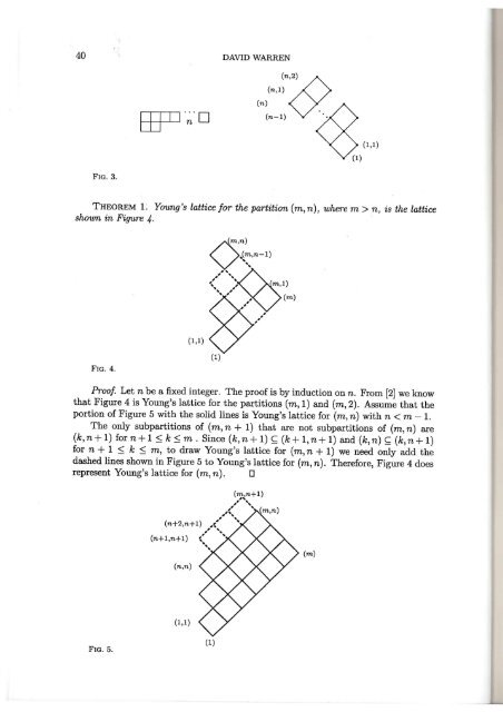
THEOREM 1. Young 's lattice for the partition (m, n), where m > n, is the lattice
shown in Figure 4.
FIG. 4.
(1,1) 8>/
~n)
vs{~·n-1)
, ..
': ~ (m,1)
.. ,
.... ,' , (m)
(1)
Proof Let n be a fixed integer. The proof is by induction on n. From [2] we know
that Figure 4 is Young's lattice for the partitions (m, 1) and (m, 2). Assume that the
portion of Figure 5 with the solid lines is Young's lattice for (m, n) with n < m- 1.
The only subpartitions of ( m, n + 1) that are not subpartitions of ( m, n) are
(k,n+ 1) for n+ 1::; k::; m. Since (k,n+ 1) ~ (k+ 1,n+ 1) and (k,n) ~ (k,n+ 1)
for n + 1 ::; k ::; m, to draw Young's lattice for (m, n + 1) we need only add the
dashed lines shown in Figure 5 to Young's lattice for (m, n). Therefore, Figure 4 does
represent Young's lattice for (m, n). 0
(~,n+1)
, ..
" (m,n)
, ..
,,'t'
..
(n+2,n+1) ,,,(: .. ,
(n+l,n+l) (. 1 '
....,
(n,n)
(m)
FIG. 6.
(1)
Once we found the general forms of partitions with two-dimensional Young's
lattices, we began looking at the conjugates of these partitions and their representative
lattices. The conjugate partition of a given partition is the partition obtained by
switching the rows and columns of Ferrer's diagram for the given partition. To switch
between a lattice and its conjugate we developed different numbering grids. The two
dimensional lattices are obtained from three general types of partitions. The first is
a partition with exactly one row or its conjugate with exactly one column in Ferrer's
diagram. Since Young's lattices of these partitions are single chains, they can be
drawn on any of the following grids.
The second type of partition is one with exactly two rows and any number of
columns or its conjugate with exactly two columns and any number of rows. In this
case, we need two different labelings (grids) when converting between a lattice and
its conjugate.
First, consider the partition with exactly two rows. We will label the spine of
the lattice as the line connecting the subpartitions of the form ( n, n - 1). The origin
of the lattice is the position of the subpartition (1). Labeling from the origin, each
time we move one position up and to the right, we add one to the first row of the
subpartition. Each time we move one position up and to the left, we add one to the
second row of the subpartition (as long as in the partition ( x, y), x 2: y) as shown in
Figure 7.
(5)
FIG. 7.
FIG. 5.
(1,1)
(1)
Now we will consider the conjugate, the partition with exactly two columns. The
spine of this lattice is the line connecting the subpartitions of the form (2, 2, ... , 2, 1)
with n rows. The origin of this lattice is also the position of the subpartition (1).
Labeling from the origin, each time we move one position up and to the left we add