Vol. 11 No 1 - Pi Mu Epsilon

42 DAVID WARREN
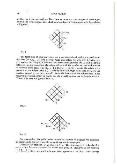
another row to the subpartition. Each time we move one position up and to the right,
we add one to the highest row which does not have a 2 (two squares) in it as shown
in Figure 8.
FIG. 8.
The third type of partition which has a two dimensional lattice is a partition of
the form (m, 1, 1, ... , 1) with n rows. With this lattice, we only need to define one
grid system, but this grid is different than either of the previous two. The spine of this
lattice is the line connecting the subpartitions with the number of rows and number
of columns being equal (i.e.: (2, 1), (3, 1, 1), (4, 1, 1, 1), etc.). Again, the origin is the
position of the subpartition (1). Labeling from the origin each time we move one
position up and to the right, we add one to the first row of the subpartition. Each
time we move one position up and to the left, we add another row to the subpartition.
This can be seen in Figures 9 and 10.
YOUNG'S LATTICES 43
to rows in the conjugate, we can see that this step gives us the correct number of entries
in the conjugate partition.
The second step is to take the second entry, y, and add one to each of the first y
1 2 3 y-1 Y y+1 X
entries of the x-tuple. This gives us the partition 2, 2, 2,... 2 , 2, 1 , ... 1. This step
takes they elements in the second row of the original partition and changes them into
they elements in the second column of the conjugate. Here again we get the correct
number of entries in the conjugate partition.
Note that this pattern holds for every position in ann-tuple partition.
With this algorithm, we can determine the conjugate of any subpartition in a
lattice. Using the appropriate grid, we can then develop the conjugate lattice.
THEOREM 3. The conjugate of a particular lattice is found by reflection about the
spine.
As we were trying to find all the general forms of partitions and their lattices,
we ran into a little problem when we looked at the partition (3, 2, 1) As it turned
out, this is the basic partition with a three dimensional lattice. The lattice for this
partition is shown in Figure 11.
Working with this partition, we noticed a general pattern that led us to the
following theorem.
(5)
FIG. 11.
THEOREM 4. Young's lattice for the partition (m, 2, 1, . .. , 1) with n rows is shown
in Figure 12.
FIG. 9.
(1,1,1, ... ,1)
(1)
FIG. 12.
FIG. 10.
Once we defined the grids needed to convert between conjugates, we developed
an algorithm to convert a specific subpartition into its conjugate.
Consider the partition (x, y) where x ~ y. The first step is to take the first
entry, x, and form an x-tuple with a one in each position. This gives us the partition
1 2 3 X
(1, 1, 1, ... 1). Since each position in a partition represents a row, and columns change
Proof. We first show that Young's lattice of the partition (m, 2, 1) is displayed
in Figure 13 by the thicker lines. We proceed by induction on m. By Figure 11,
this is true for (3, 2, 1). Now assume that the lattice for the partition (m, 2, I) is as
shown in Figure 13 by the thicker lines. The only subpartitions of (m + 1, 2, 1) that
are not subpartitions of (m, 2, 1) are (m + 1), (m + 1, 1), (m + 1, 2), (m + 1, 1, 1),
and (m + 1, 2, 1). As pictured by the dashed lines in Figure 13, these subpartitions
connect, as desired, to the lattice for (m, 2, 1).