Design Optimization of Hierarchically Decomposed Multilevel ...

More documents

Recommendations

Info

Finally, to compute moments, we integrate numerically, using spline interpolation to estimate response values that lie between the available PDF values. As will be shown by means of several analytical examples, this method is quite accurate. 3.3 Examples The MVFOSM-based and AMV-based methods were used to estimate the first two moments of several nonlinear analytical expressions. All random variables were assumed to be normal. Test functions and input statistics are presented in Table 1 and results are summarized in Table 2. One million samples were used for the Monte Carlo simulations. 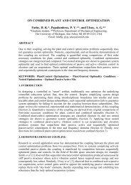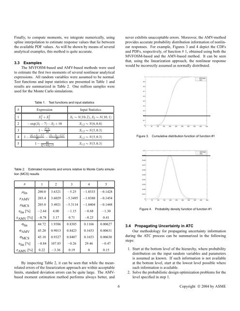never exhibits unacceptable errors. Moreover, the AMV-method provides accurate probability distribution information of nonlinear responses. For example, Figures 3 and 4 depict the CDFs and PDFs, respectively, of function # 1, obtained using both the MVFOSM-based and the AMV-based method. It can be seen that, using the linearization approach, the nonlinear response would be incorrectly assumed as normally distributed. Table 1. Test functions and input statistics # Expression Input Statistics 1 X 2 1 + X2 2 X 1 ∼ N(10,2), X 2 ∼ N(10,1) 2 −exp(X 1 − 7) − X 2 + 10 X 1,2 ∼ N(6,0.8) 3 1 − X 2 1 X 2 20 X 1,2 ∼ N(5,0.3) 4 1 − (X 1+X 2 −5) 2 30 − (X 1−X 2 −12) 2 30 X 1,2 ∼ N(5,0.3) 5 1 − 80 X 2 1 +8X 2+5 X 1,2 ∼ N(5,0.3) Figure 3. Cumulative distribution function of function #1 Table 2. Estimated moments and errors relative to Monte Carlo simulation (MCS) results # 1 2 3 4 5 µ lin 200.0 3.6321 −5.25 −1.0333 −0.1428 µ AMV 203.4 3.6029 −5.3495 −1.0380 −0.1454 µ MCS 205.0 3.4921 −5.3114 −1.0404 −0.1448 ε lin [%] −2.44 4.00 −1.15 −0.68 −1.30 ε AMV [%] −0.78 3.17 0.71 −0.23 0.41 σ lin 44.72 1.9386 0.8385 0.1166 0.00627 σ AMV 45.20 0.9013 0.8423 0.1653 0.00631 σ MCS 45.10 0.9327 0.8407 0.1653 0.00630 ε lin [%] −0.84 107.85 −0.26 29.46 −0.47 ε AMV [%] 0.22 −3.36 0.19 0 0.15 By inspecting Table 2, it can be seen that while the meanrelated errors of the linearization approach are within acceptable limits, standard deviation errors can be quite large. The AMVbased moment estimation method performs always better, and Figure 4. Probability density function of function #1 3.4 Propagating Uncertainty in ATC Our methodology for propagating uncertainty information during the ATC process can be summarized in the following steps: 1. Start at the bottom level of the hierarchy, where probability distribution on the input random variables and parameters is assumed as known. If such information is not available at the bottom level, start at the lowest level possible where such information is available. 2. Solve the probabilistic design optimization problems for the level specified in step 1. 6 Copyright © 2004 by ASME
3. Use the approach described in Section 3.2 to obtain distribution information for the response variables that are inputs to higher-level (“parent”) problems. 4. Using the information obtained at step 3, solve the parent problems. Note that the CDFs and PDFs of lower-level (“children”) responses that constitute optimization variables in the parent problems are required for solving these problems correctly. Second moment (variance) information alone is inadequate to guarantee proper solution process and uncertainty propagation throughout the hierarchy (as opposed, e.g., to “single”-element robust design optimization). 5. Move your way to the top of the hierarchy. 6. Once you have reached the top-level problem start moving towards the bottom using previous solutions to update parameters as shown in Figure 2. 7. Keep iterating until all ε values in all problems in the hierarchy have been reduced as much as possible, i.e., have converged to a steady state value. Note that the ε variables are deterministic, as are the constraints they appear in. While uncertainties are taken into account in the probabilistic design constraints, the non-deterministic ATC process aims at coordinating values of shared variables and responses in an average sense. Note that since the linearization approach is sufficiently accurate for estimating expected values, it can be used to reduce computational cost. However, the AMV-based method is so efficient, that it is suggested for use in estimating expected values to improve accuracy and thus, possibly, the convergence rate of the ATC process. 4 METAMODELING FOR SIMULATION-BASED DE- SIGN UNDER UNCERTAINTY The state-of-the-art analytical reliability analysis methods are gradient based. When simulations are used to compute responses, as is the case in our following example (Section 5), numerical noise can occur. In addition, simulations tend to be computationally expensive. Computational cost is then aggregated during optimization and reliability analysis. Use of metamodels (or surrogate models, or response surfaces) is the established remedy to address the above issues. However, metamodels introduce additional errors to the ones already existing due to lack of knowledge, inability to represent physics with mathematical expressions, incomplete information, numerical arithmetic errors, uncertainty, and its propagation, as illustrated in the following expression R = f (x) + ε physics + ε modeling + ε metamodeling + ε data + ε numerics + ε uncertainty + ε uncertainty propagation . Approximations and errors are a reality that we must acknowledge even if we are not in a position to eliminate completely. There is no meaning in driving just one error down to zero if any of the remaining ones are still relatively large [36]. Our point is that if metamodels must be used, they must be associated with small errors relative to other error sources. Traditional response surface methodology using Design of Experiments (DOE) techniques [37, 38], such as fractional factorials, central composite, Plackett-Burman, and Box-Behnken designs, is usually computationally efficient. However, it often becomes inadequate in nonlinear multivariate metamodeling of complex simulation models. In traditional parametric regression, the metamodel functional form is assumed known (e.g., polynomials in the conventional least-squares regression). The goal of regression analysis is to determine the parameter values of the assumed functional form, so that the generated metamodel best fits the provided data set. A linear or nonlinear parametric metamodel is likely to produce good approximations only when the assumed functional form is close to the true underlying function. For this reason, nonparametric regression techniques [39, 40], along with the progressive space-filling sampling [41, 42], have attracted a growing interest. They only use a few general assumptions about the functional form of the metamodel, such as its smoothness properties. The functional form is not prespecified, but determined instead from the available data. The nonparametric approach is therefore, more flexible and is likely to produce accurate nonlinear approximations even if the true underlying function form is totally unknown. Many nonparametric techniques have been proposed for univariate modeling, such as smoothing splines and local polynomial fitting [43, 44]. They can be easily extended to multivariate cases. As a more general case of smoothing splines, nonparametric regression methods using Gaussian process models (similar to Kriging in spatial statistics) and radial basis functions (RBF), have been used to fit data from computer experiments [45–47]. The local polynomial fitting and Kriging/RBF techniques have demonstrated better predictive performance than the parametric regression techniques [48]. Their main advantage is an automated metamodeling process, in which the hyper-parameters in local polynomial fitting and Kriging can be determined by minimizing the metamodel cross-validation error and maximizing the likelihood function, respectively. Local polynomial fitting, using the cross-validated moving least squares (CVMLS) method [39, 40], is used in this paper. 4.1 Optimal Symmetric Latin Hypercube Sampling In order to construct a metamodel using the CVMLS method, an appropriate sampling technique is necessary, which preferably uses a modest number of samples with the potential to explore nonlinear input/output relationships. Previous studies have found that uniformity is the most important criterion, while the space-filling uniform design is preferable [41, 42]. The opti- 7 Copyright © 2004 by ASME
Page 1 and 2: Proceedings of DETC’04 ASME 2004
Page 3 and 4: level i=0 system j=1 optimization i
Page 5: and Var[R] = σ 2 R ≈ n ∑ i=1 (
Page 9 and 10: estimated from solving an unconstra
Page 11 and 12: One million samples were generated
Page 13: matikas, N.F. Michelena, Z.S. Filip

Design Optimization of Hierarchically Decomposed Multilevel ...

You also want an ePaper? Increase the reach of your titles

Delete template?

Save as template?