A State-Space Representation Model and Learning Algorithm for ...

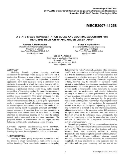
Proceedings of IMECE072007 ASME International Mechanical Engineering Congress and ExpositionNovember 11-15, 2007, Seattle, Washington, USAIMECE2007-41258A STATE-SPACE REPRESENTATION MODEL AND LEARNING ALGORITHM FORREAL-TIME DECISION-MAKING UNDER UNCERTAINTYAndreas A. MalikopoulosPanos Y. PapalambrosDepartment of Mechanical EngineeringDepartment of Mechanical EngineeringUniversity of MichiganUniversity of MichiganAnn Arbor, Michigan 48109, U.S.AAnn Arbor, Michigan 48109, U.S.Aamaliko@umich.edupyp@umich.eduDennis N. AssanisDepartment of Mechanical EngineeringUniversity of MichiganAnn Arbor, Michigan 48109, U.S.Aassanis@umich.eduABSTRACTModeling dynamic systems incurring stochasticdisturbances for deriving a control policy is a ubiquitous task inengineering. However, in some instances obtaining a model ofa system may be impractical or impossible. Alternativeapproaches have been developed using a simulation-basedstochastic framework, in which the system interacts with itsenvironment in real time and obtains information that can beprocessed to produce an optimal control policy. In this context,the problem of developing a policy for controlling the system’sbehavior is formulated as a sequential decision-makingproblem under uncertainty. This paper considers real-timesequential decision-making under uncertainty modeled as aMarkov Decision Process (MDP). A state-space representationmodel is constructed through a learning mechanism and is usedto improve system performance over time. The model allowsdecision making based on gradually enhanced knowledge ofsystem response as it transitions from one state to another, inconjunction with actions taken at each state. A learningalgorithm is implemented realizing in real time the optimalcontrol policy associated with the state transitions. Theproposed method is demonstrated on the single cart-polebalancing problem and a vehicle cruise control problem.Keywords: sequential decision-making under uncertainty,Markov Decision Process (MDP), reinforcement learning,learning algorithms, inverted pendulum, vehicle cruise control1. INTRODUCTIONDeriving a control policy for dynamic systems is an offlineprocess in which various methods from control theory areutilized iteratively. These methods aim to determine the policythat satisfies the system’s physical constraints while optimizingspecific performance criteria. A challenging task in this processis to derive a mathematical model of the system’s dynamics thatcan adequately predict the response of the physical system toall anticipated inputs. Exact modeling of complex engineeringsystems, however, may be infeasible or expensive. Viablealternative methods have been developed enabling the real-timeimplementation of control policies for systems when anaccurate model is not available. In this framework, the systeminteracts with its environment, and obtains informationenabling it to improve its future performance by means ofrewards associated with control actions taken. This interactionportrays the learning process conveyed by the progressiveenhancement of the system’s “knowledge” regarding the courseof action (control policy) that maximizes the accumulatedrewards with respect to the system’s operating point (state).The environment is assumed to be non-deterministic; namely,taking the same action in the same state on two different stages,the system may transit to a different state and receive adissimilar reward in the subsequent stage. Consequently, theproblem of developing a policy for controlling the system’sbehavior is formulated as a sequential decision-makingproblem under uncertainty.Dynamic programming (DP) has been widely employed asthe principal method for analysis of sequential decision-makingproblems [1]. Algorithms, such as value iteration, and policyiteration, have been extensively utilized in solvingdeterministic and stochastic optimal control problems, Markovand semi-Markov decision problems, min-max controlproblems, and sequential games. However, the computationalcomplexity of these algorithms in some occasions may beprohibitive and can grow intractably with the size of the1 Copyright © 2007 by ASME

problem and its related data, referred to as the DP “curse ofdimensionality” [2]. In addition, DP algorithms require therealization of the conditional probabilities of state transitionsand the associated rewards, implying a priori knowledge of thesystem dynamics.Alternative approaches for solving sequential decisionmakingproblems under uncertainty have been primarilydeveloped in the field of Reinforcement Learning (RL) [3, 4].RL has aimed to provide simulation-based algorithms, foundedon DP, for learning control policies of complex systems, whereexact modeling is infeasible or expensive [5]. A majorinfluence on research leading to current RL algorithms hasbeen Samuel’s method [6, 7], used to modify a heuristicevaluation function for deriving optimal board positions in thegame of checkers. In this algorithm, Samuel represented theevaluation function as a weighted sum of numerical featuresand adjusted the weights based on an error derived fromcomparing evaluations of current and predicted board positions.This approach was refined and extended by Sutton [8, 9] tointroduce a class of incremental learning algorithms, TemporalDifference (TD). TD algorithms are specialized for derivingoptimal policies for incompletely known systems, using pastexperience to predict their future behavior. Watkins [10, 11]extended Sutton’s TD algorithms and developed an algorithmfor systems to learn how to act optimally in controlled Markovdomains by explicitly utilizing the theory of DP. A strongcondition implicit in the convergence of Q-learning to anoptimal control policy is that the sequence of stages that formsthe basis of learning must include an infinite number of stagesfor each initial state and action. However, Q-learning isconsidered the most popular and efficient model-free learningalgorithm in deriving optimal control policies in Markovdomains [12]. Schwartz [13] explored the potential of adaptingQ-learning to an average-reward framework with his R-learning algorithm; Bertsekas and Tsitsiklis [3] presented asimilar to Q-learning average-reward algorithm. Mahadevan[14] surveyed reinforcement-learning average-rewardalgorithms and showed that these algorithms do not alwaysproduce bias-optimal control policies.Although many of these algorithms are eventuallyguaranteed to find optimal policies in sequential decisionmakingproblems under uncertainty, their use of theaccumulated data acquired over the learning process isinefficient, and they require a significant amount of experienceto achieve good performance [12]. This requirement arises dueto the formation of these algorithms in deriving optimalpolicies without learning the system models en route.Algorithms for computing optimal policies by learning themodels are especially important in applications in which realworldexperience is considered expensive. Sutton’s Dynaarchitecture [15, 16] exploits strategies which simultaneouslyutilize experience in building the model and adjust the derivedpolicy. Prioritized sweeping [17] and Queue-Dyna [18] aresimilar methods concentrating on the interesting subspaces ofthe state-action space. Barto et al. [19] developed anothermethod, called Real-Time Dynamic Programming (RTDP),referring to the cases in which concurrently executing DP andcontrol processes influence one another. RTDP focuses thecomputational effort on the state-subspace that the system ismost likely to occupy. This method is specific to problems inwhich the system needs to achieve particular goal states and theinitial cost of every goal state is zero.This paper considers the problem of deriving optimalpolicies in real-time sequential decision-making underuncertainty that can be modeled as a Markov Decision Process(MDP). A state-space representation model is constructedthrough a learning mechanism and is used to improve systemperformance over time. The model accumulates graduallyenhanced knowledge of system response as it transitions fromone state to another, in conjunction with actions taken at eachstate. A learning algorithm is implemented realizing in real timethe optimal course of action (control policy) associated with thestate transitions. The major difference between the proposedmethod and the existing RL algorithms is that the latter consistsof evaluation functions attempting to successively approximatethe Bellman equation [20]. The proposed real-time learningmethod, on the contrary, utilizes an evaluation function whichconsiders the expected reward that can be achieved by statetransitions forward in time. This approach is especiallyappealing to learning engineering systems in which the initialstate is not fixed, and recursive updates of the evaluationfunctions to approximate the Bellman equation would demandsignificant amount of experience to achieve the desired systemperformance.In the following section the mathematical framework formodeling sequential decision-making problems underuncertainty is presented and the predictive optimal decisionmakinglearning method is introduced. The performance of theproposed method is demonstrated on the single cart-polebalancing problem, in Section 3 and, on a vehicle cruisecontrolproblem, in Section 4. Conclusions are presented inSection 5.2. PROBLEM FORMULATIONA large class of sequential decision-making problemsunder uncertainty can be modeled as a Markov DecisionProcess (MDP). MDP, extensively covered by Puterman [21],provides the mathematical framework for modeling decisionmakingin situations where outcomes are partly random andpartly under the control of the decision maker. Decisions aremade at points of time referred to as decision epochs, and thetime domain can be either discrete or continuous. The focus ofthis paper is on discrete-time decision-making problems.The Markov decision process model consists of fiveelements: (a) decision epochs; (b) states; (c) actions; (d) thetransition probability matrix; and (e) the transition rewardmatrix. In this framework, the decision maker is faced with theproblem of influencing system behavior as it evolves over time,by making decisions (choosing actions). The objective of thedecision maker is to select the course of action (control policy)2 Copyright © 2007 by ASME

which causes the system to perform optimally with respect tosome predetermined optimization criterion. Decisions mustanticipate rewards (or costs) associated with future systemstates-actions.At each decision epoch, the system occupies a state s ifromthe finite set of all possible system states SS = { si| i = 1,2,..., N}, N∈N .(1)In this state s i∈S , the decision maker has available a set ofallowable actions, α ∈As(i), As (i)⊆A , where A is the finiteaction spaceA = ∪ sA( s ).i∈Si(2)The decision-making process occurs at each of a sequenceof decision epochs T = 0,1, 2,..., M,M ∈N . At each epoch,the decision maker observes a system’s state s i∈S , andexecutes an action α ∈ A( s i), from the feasible set of actionsAs ( i) ⊆ A at this state. At the next epoch, the system transits tothe state sj∈S imposed by the conditionalprobabilities ps (j| si, α ), designated by the transitionprobability matrix P(⋅,⋅). The conditional probabilities ofP(⋅,⋅), p : S × A →[0,1], satisfy the constraintN∑ ps (j| si, α) = 1.(3)j=1Following this state transition, the decision maker receives areward associated with the action α, Rs (j| si, α ), R:S × A → Ras imposed by the transition reward matrix R(⋅,⋅). The states ofan MDP possess the Markov property, stating that theconditional probability distribution of future states of theprocess depends only upon the current state and not on any paststates, i.e., it is conditionally independent of the past states (thepath of the process) given the present state. Mathematically, theMarkov property states thatpX (n+ 1= sj | Xn = si, Xn− 1= si−1,..., X0 = s0)=(4)= pX ( = s | X = s).n+1 j n i2.1 Optimal Policies and Performance CriteriaThe solution to an MDP can be expressed as an admissiblecontrol policy such that a given performance criterion isoptimized over all admissible policies Π. An admissible policyconsists of a sequence of functionsπ = { µ0, µ1,..., µ M},(5)where µ Tmaps states s iinto actions α = µ T( s i) and is suchthat µT( si) ∈A( si), ∀si∈S.Consequently, given an initial state at decision epoch T = 0,si, and an admissible policy π = { µ0, µ1,..., µ M}, the expectedaccumulated undiscounted value of the rewards of the decisionmaker is given by the Bellman optimality equationM −1i N N−1 µN−1T j iµiT = 0V( s ) = E{ R( s | s , ( s )) +∑ V ( s | s , ( s ))}, (6)∀si, sj∈ S , i, j = 1,2,..., N, N∈N.In the finite-horizon context the decision maker shouldmaximize the accumulated value for the next M epochs. Anoptimal policy π * ∈Π is one that maximizes the overallexpected accumulated value of the rewardsV ( s ) = max V ( s ).(7)∗πiπ∈Ππ i∗ ∗ ∗ ∗Consequently, the optimal policy π = { µ0, µ1,..., µ M} for theM-decision epoch sequence is∗π = arg max V ∗ ( s i).(8)π∈ΠThe finite-horizon model is appropriate when the decisionmaker’s“lifetime” is known, namely, the terminal epoch of thedecision-making sequence. For problems with a very largenumber of decision epochs, however, the infinite-horizonmodel is more appropriate. In this context, the overall expectedundiscounted reward is:Vπ* ( si) = lim max Vπ( si).(9)M →∞ π∈ΠThis relation is valuable computationally and analytically, andit holds under certain conditions [22].2.2 Predictive Optimal Decision-Making State-SpaceRepresentationThe predictive optimal decision-making (POD) learningmethod consists of a new state-space system representation anda learning algorithm. The state-space representationaccumulates gradually enhanced knowledge of the system’stransition from each state to another in conjunction with actionstaken for each state. This knowledge is expressed in terms of anexpected evaluation function associated with each state. Whilethe model’s knowledge is advanced, the learning algorithmrealizes, at each decision epoch, the course of action thatguarantees at least a minimum value of the overall reward forboth the current state and the subsequent states.The major difference between the proposed learningmethod and the existing RL methods is that the latter consistsof evaluation functions attempting to successively approximatethe Bellman equation, Eq. (6). These evaluation functionsassign to each state the total reward expected to accumulateover time starting from a given state when a policy π isemployed. The proposed real-time learning method, on thecontrary, utilizes an evaluation function which considers theexpected reward that can be achieved by state transitionsforward in time. This approach is especially appealing tolearning engineering systems in which the initial state is notfixed [23, 24], and recursive updates of the evaluationfunctions to approximate Eq.(6) would demand a huge numberof iterations to achieve the desired system performance.The new state-space representation defines the PODdomain S . It is implemented by a mapping H from theπ3 Copyright © 2007 by ASME

Cartesian product of the finite state space and action space ofthe MDP:H: ( S× A) × ( S× A) →S , (10)where S = { si| i = 1,2,..., N},N∈Ndenotes the Markov statespace, and A = ∪ sAs ( ),i∈Si∀si∈Sstands for a finite actionspace. This mapping generates an indexed family ofsubsets, S s i, for each state s i∈S , defined as PredictiveRepresentation Nodes (PRNs). Each PRN is constituted by aiset of POD states, s ∈S ,msiiSs = { s| , 1,2,..., , | | }i mi m= N N = S ∈N , (11)Each POD state s i ∈S messentially represents a Markov statetransition from s i∈S to s m∈S . PRNs partition the PODdomain insofar as the POD underlying structure captures thestate transitions in the Markov domain. Consequently, a PRN isdefined asNi im m i m ∑ m iµiµ ( si) ∈A( si)m=1S s = { s | s ≡ s → s , p ( s | s , ( s )) = 1, N = | S |},i∀si, sm ∈S , ∀µ( si) ∈A( si),(12)the union of which defines the POD domainS= ∪ i s i, withs∈SS (13)s ims i∩ S =∅.(14)Ssim∈s is iEach PRN, S , corresponds to a Markov state, si∈S , andportrays all possible transitions occurring from this state s i tothe other states s m∈S . PRNs, constituting the fundamentalaspect of the POD state representation, provide an assessmentof the Markov state transitions along with the actions executedat each state. This assessment aims to establish a necessaryembedded property of the new state representation so as toconsider the potential transitions that can occur in subsequentdecision epochs. The assessment is expressed by means of theiPRN value, Rs ( s| ( ))i mµ si, which accounts for the maximumaverage expected reward that can be achieved by transitionsoccurring inside a PRN. Consequently, the PRN value isdefined asN⎛⎞⎜∑p( sm | si, µ ( si)) ⋅ R( sm | si, µ ( si))⎟im=1Rs ( s| ( )) max ,i mµ si= ⎜⎟µ ( si) ∈A⎜N⎟⎜⎟⎝⎠i∀s m∈S, ∀si, sm ∈S, ∀µ( si) ∈ A( si),and N = | S |. (15)The PRN value is exploited by POD state representation asan evaluation metric to estimate the subsequent Markov statetransitions. The estimation property is founded on theassessment of POD states by means of an expected evaluationi ifunction, R ( s, µ ( s )), defined asPRN m i{i iRPRN ( sm, µ ( si )) = p( sm | si , µ ( si )) ⋅ R( sm | si , µ ( si)) +(16)m+ Rs ( s| ( ))},m jµ smi m∀sm, sj∈S, ∀si, sm ∈S, ∀µ ( si) ∈A( si), ∀µ( sm) ∈A( sm).Consequently, employing the POD evaluation function throughiEq. (16), each POD state, sm∈S s , is comprised of an overallireward corresponding to: (a) the expected reward of transitingfrom state s i to s m (implying also the transition from the PRNSs itoSs m); and (b) the maximum average expected rewardwhen transiting from s m to any other Markov state (transitionoccurring into S s m).While the system interacts with its environment, the PODmodel learns the system dynamics in terms of the Markov statetransitions. The POD state representation attempts to provide aprocess in realizing the sequences of state transitions thatoccurred in the Markov domain, as infused in PRNs. Thedifferent sequences of the Markov state transitions are capturedby the POD states and evaluated through the expectedevaluation functions given in Eq. (16). Consequently, thehighest value of the expected evaluation function at each PODstate essentially estimates the subsequent Markov statetransitions with respect to the actions taken. As the process isstochastic, however, it is still necessary for the real-timelearning method to build a decision-making mechanism of howto select actions.The learning performance is closely related to theexploration-exploitation strategy of the action space. Moreprecisely, the decision maker has to exploit what is alreadyknown regarding the correlation involving the admissible stateactionpairs that maximize the rewards, and also to explorethose actions that have not yet been tried for these pairs toassess whether these actions may result in higher rewards. Abalance between an exhaustive exploration of the environmentand the exploitation of the learned policy is fundamental toreach nearly optimal solutions in few decision epochs and,thus, enhancing the learning performance. This explorationexploitationdilemma has been extensively reported in theliterature. Iwata et al. [25] proposed a model-based learningmethod extending Q-learning and introducing two separatedfunctions based on statistics and on information by applyingexploration and exploitation strategies. Ishii et al. [26]developed a model-based reinforcement learning methodutilizing a balance parameter, controlled through variation ofaction rewards and perception of environmental change. Chan-Geon et al. [27] proposed an exploration-exploitation policy inQ-learning consisting of an auxiliary Markov process and theoriginal Markov process. Miyazaki et al. [28] developed aunified learning system realizing the tradeoff betweenexploration and exploitation. Hernandez-Aguirre et al. [29]analyzed the problem of exploration-exploitation in the contextof the probably approximately correct framework and studiedwhether it is possible to give bounds on the complexity of the4 Copyright © 2007 by ASME

“neural-fuzzy BOXES” control system by neural networks andutilized reinforcement learning for the training. Jeen-Shing etal. [33] proposed a defuzzification method incorporating agenetic algorithm to learn the defuzzification factors. Mustaphaet al. [34] developed an actor-critic reinforcement learningalgorithm represented by two adaptive neural-fuzzy systems. Siet al. [35] proposed a generic on-line learning control systemsimilar to Anderson’s utilizing neural networks and evaluated itthrough its application to both a single and double cart-polebalancing problem. The system utilizes two neural networks,and employs the action- dependent heuristic dynamicprogramming to adapt the weights of the networks.In the implementation of the POD on the single invertedpendulum presented here, two major variations are considered:(a) a single look-up table-based representation is employed forthe controller to develop the mapping from the system’sMarkov states to optimal actions, and (b) two system’s statevariables are selected to represent the Markov state. The latterintroduces uncertainty and thus a conditional probabilitydistribution associating the state transitions with respect to theactions taken. Consequently, the POD method is evaluated inderiving the optimal policy (balance control policy) in asequential decision making problem under uncertainty.The governing equations, derived from the free bodydiagram of the system, shown in Figure 2, are:2( M + m) x + bx + mLϕcosϕ− mL ϕ sin ϕ = U , (19)2mLx cos ϕ+ ( I + mL ) ϕ+ mgL sinϕ= 0, (20)N secwhere M = 0.5 kg, m = 0.2 kg, b=0.1m2 mI = 0.006 kg m , g = 9.81 ,and L = 0.3 m.2secThe goal of the learning controller is to realize in real timethe force, U, of a fixed magnitude to be applied either to theright or the left direction so that the pendulum stands balancedwhen released from any angle, φ, between 3° and -3°. Thesystem is simulated by numerically solving the nonlineardifferential equations (19) and (20) employing the explicitRunge-Kutta method with a time step of τ =0.02 sec. Thesimulation is conducted by observing the system’s states andexecuting actions (control force U) with a sample rate T =0.02sec (50 Hz). This sample rate defines a sequence of decisionmakingepochs, T = 0,1, 2,..., M,M ∈N .The system is fully specified by four state variables: (a) theposition of the cart on the track, x()t ; (b) the cart velocity,x() t ; (c) the pendulum’s angle with respect to the verticalposition, ϕ () t ; and (d) the angular velocity, ϕ () t . However, toincorporate uncertainty, the Markov states are selected to beonly the pair of the pendulum’s angle and angular velocity,namely, the finite state space S, in Eq. (1) is defined asS = { s | s = ( ϕ, ϕ)}.(21)iiUN HN VMxxbxIϕ 2LϕmgN HFigure 2. Free body diagram of the system.IϕmI,Consequently, at state si∈S and executing a control forcevalue, U(s i ), the system will end up at state s j∈S with aconditional probably ps (j| si, Us (i)). The control force, U(s i ),selects values from the finite set A, defined asA = As (i) = [ − 3 N,3 N], where i= 1, 2,..., N, N=| S | . (22)The decision-making process occurs at each of a sequence ofepochs T = 0,1, 2,..., M,M ∈ N . At each decision epoch, thelearning controller observes the system’s state s i∈S , andexecutes a control force value U( si) ∈ A( si). At the nextdecision epoch, the system transits to another statesj∈S imposed by the conditional probabilitiesps (j| si, Us (i)), and receives a numerical reward (thependulum’s angle φ).The inverted pendulum is simulated repeatedly fordifferent initial angles, φ, between 3° and -3° utilizing the PODlearning method. The simulation lasts for 50 sec and eachcomplete simulation defines one iteration. If at any instantduring the simulation, the pendulum’s angle, φ, becomesgreater than 3° or less than -3°, this constitutes a failure,denoted by stating that there was one iteration associated with afailure. If, however, no failure occurs during the simulation,this is denoted by stating that there was one iteration associatedwith no failure.3.2 Simulation ResultsAfter completing the learning process, the controller employingthe POD learning method realizes the balance control policy ofthe pendulum, as illustrated in Figure 3. In some instances,however, the system’s response demonstrates some overshootsor delays during the transient period, shown in Figure 4. Thiscan be handled by a denser parameterization of the state-spaceor adding a penalty in long transient responses. The efficiencyof the POD learning method in deriving the optimal balancecontrol policy that stabilizes the system is illustrated in Figure5. It is noted that after POD realizes the optimal policy in 749failures and, afterwards, as the number of iterations continuesno further failures occur.N Vx6 Copyright © 2007 by ASME

Phi [deg]43210-1-2-3Simulation of the Controlled Pendulum with POD-40 10 20 30 40 50time [sec]Figure 3. Simulation of the system after learning the balancecontrol policy with POD for different initial conditions.Phi [deg]3210-1-2Simulation of the Controlled Pendulum with POD-30 0.1 0.2 0.3 0.4 0.5 0.6 0.7 0.8time [sec]Figure 4. Simulation of the system after learning the balancecontrol policy with POD for different initial conditions (zoomin).Failures800700600500400300200100Number of Failures of POD in derivingthe balance control policy00 0.5 1 1.5 2Iterationsx 10 4Figure 5. Number of failures until POD derives the balancecontrol policy.4. CASE STUDY TWO4.1 Vehicle Cruise ControlThe POD real-time learning method introduced in theprevious sections is now applied to a vehicle cruise-controlproblem. Cruise control automatically regulates the vehicle’slongitudinal velocity by suitably adjusting the gas pedalposition. A vehicle cruise-control system is activated by thedriver who desires to maintain a constant speed in longhighway driving. The driver activates the cruise controllerwhile driving at a particular speed, which is then recorded asthe desired or set-point speed to be maintained by thecontroller. The main goal in designing a cruise controlalgorithm is to maintain vehicle speed smoothly but accurately,even under large variation of plant parameters (e.g., thevehicle’s varying mass in terms of the number of passengers)and road grade. In the case of passenger cars, however, vehiclemass may change noticeably but is within a small range.Therefore, powertrain behavior might not vary significantly.The objective of the POD learning cruise controller is torealize in real time the control policy (gas pedal position) thatmaintains the vehicle speed as set by the driver under a greatrange of different road grades. Implementing learning vehiclecruise controllers has been addressed previously employinglearning and active control approaches. Zhang et al. [36]implemented learning control based on pattern recognition toregulate in real time the parameters of an PID cruise controller.Shahdi et al. [37] proposed an active learning method to extractthe driver's behavior and to derive control rules for a cruisecontrol system. However, no attempt has been reported inimplementing a learning automotive vehicle cruise controllerutilizing the principle of reinforcement learning, i.e., enablingthe controller to improve its performance over time by learningfrom its own failures through a reinforcement signal from theexternal environment, and thus, attempting to improve futureperformance.The software package enDYNA by TESIS [38], suitable forreal-time simulation of internal combustion engines, is used toevaluate the performance of the POD learning cruise controller.The software simulates the longitudinal vehicle dynamics witha highly variable drive train including the modules of starter,brake, clutch, converter, and transmission. In the driving modethe engine is operated by means of the usual vehicle controlelements just as a driver would do. In addition, a mechanicalparking lock and the uphill grade can be set. The driver modelis designed to operate the vehicle at given speed profiles(driving cycles). It actuates the starter, accelerator, clutch andbrake pedals according to the profile specification, and alsoshifts gears. In this example, an existing vehicle model isselected representing a midsize passenger car carrying an 1.9Lturbocharged diesel engine.When activated, the learning cruise controller bypasses thedriver model and takes over the vehicle’s cruising. The Markovstates are defined to be the pair of the transmission gear and the7 Copyright © 2007 by ASME

difference between the desired and actual vehicle speed, ∆V,namely,S = { si| si= ( gear, ∆V)}.(23)The actions, α, correspond to the gas pedal position andcan take values from the feasible set A, defined asA = As (i) = [0,0.7], where i= 1, 2,..., N, N=| S | . (24)To incorporate uncertainty the vehicle is simulated in agreat range of different road grades from 0° to 10°.Consequently, at state s i∈S and executing a control action(gas pedal position), the system transits to another statesj∈S with a conditional probably ps (j| si, α ( si)), since theacceleration capability of a vehicle varies at different roadgrades. As a consequence of this state transition the systemreceives a numerical reward (difference between the desiredand actual vehicle speed).4.2 Simulation ResultsAfter completing four simulations of each road grade, the PODcruise controller realizes the control policy (gas pedal position)to maintain the vehicle’s speed at the desired set point. Thevehicle model was initiated from zero speed. The driver model,following the driving cycle, accelerated the vehicle up to40mph and at 10sec activated the POD cruise controller. Thedesired and actual vehicle speeds for three different road gradesas well as the gas pedal rates of the POD controller areillustrated in Figure 6. The small discrepancy between thedesired and actual vehicle speed before the cruise controlleractivation is due to the steady-state error of the driver’s model.However, since the desired driving cycle set the vehicle’s speedto be at 40mph, when the POD cruise controller is activatedhelps to correct this error and, afterwards, maintains thevehicle’s actual speed at the set point. The accelerator pedalposition is at different values because in the case of road grades2º and 6º the selected transmission gear is 2, shown in Figure 7,while in case of road grade 10º the selected transmission gear is1. So, at different selected gears, the accelerator pedal varies tomaintain constant vehicle’s speed. In Figure 8, the performanceof POD cruise controller is evaluated in a severe drivingscenario where the road grade changes from 0° to 10°, whilethe POD cruise controller is active. In this scenario, the POD isactivated again at 10sec when the road grade is 0°, and at 14sec the road grade becomes 10°. The engine speed and theselected transmission gear for this scenario are shown in Figure9. While the vehicle is cruising at constant speed and the roadgrade changes from 0º to 10º, the vehicle’s speed startsdecreasing after some time. Once this occurs, the self-learningcruise controller senses the discrepancy between the desiredand actual vehicle speed and commands the accelerator pedalso as to correct the error. Consequently, there is a small timedelay in the acceleration pedal command, illustrated in Figure8, which depends on vehicle inertia.Vehicle Velocity [mph]Accelerator PedalCruise Control with POD4030Driving Cycle20Grade 2 oGrade 6 o10Grade 10 o00 5 10 15 2010.500 5 10 15 20Time [sec]Figure 6. Vehicle speed and accelerator pedal rate for differentroad grades by self-learning cruise control with POD.Engine Speed [RPM]30002000Cruise Control with POD1000Grade 2 o00 5 10 Grade 15 6 o 20Grade 10 o3Transmission Gear2100 5 10 15 20Time [sec]Figure 7. Engine speed and transmission gear selection fordifferent road grades by self-learning cruise control with POD.Vehicle Velocity [mph]Accelerator PedalCruise Control with PODAt 14 sec the road grade increases from 0 o to 10 o4030Driving Cycle20Vehicle Speed1000 5 10 15 2010.500 5 10 15 20Time [sec]Figure 8. Vehicle speed and accelerator pedal rate for a roadgrade increase from 0° to 10°.8 Copyright © 2007 by ASME

Engine Speed [RPM]300020001000Transmission GearCruise Control with PODAt 14 sec the road grade increases from 0 o to 10 o00 5 10 15 2032100 5 10 15 20Time [sec]Figure 9. Engine speed and transmission gear selection for aroad grade increase from 0° to 10°.5. CONCLUDING REMARKSThis paper has presented a real-time learning method,consisting of a new state-space representation model and alearning algorithm, suited to solve sequential decision-makingproblems under uncertainty in real time. The method aims tobuild autonomous engineering systems that can learn toimprove their performance over time in stochasticenvironments. Such systems must be able to sense theirenvironments, estimate the consequences of their actions, andlearn in real time the course of action (control policy) thatoptimizes a specified objective. The major difference betweenthe POD learning method presented in this paper and theexisting reinforcement learning methods is that the firstemploys an evaluation function which does not requirerecursive iterations to approximate the Bellman equation. Thisapproach has been shown to be especially appealing to systemsin which the initial state is not fixed, and recursive updates ofthe evaluation functions to approximate the Bellman equationwould demand significant amount of experience to achieve thedesired system performance.The overall performance of the POD method in deriving anoptimal control policy was evaluated by its application to twoexamples: (a) the cart-pole balancing problem, and (b) a realtimevehicle cruise-controller development. In the firstproblem, POD realized the balancing control policy for aninverted pendulum when the pendulum was released from anyangle between 3° and -3°. In implementing the real-time cruisecontroller, the POD was able to maintain the desired vehicle’sspeed at any road grade between 0° and 10°. Future researchshould investigate the potential of advancing the POD methodto accommodate more than one decision maker in sequentialdecision-making problems under uncertainty, known as multiagentsystems [39]. These problems are found in systems inwhich many intelligent decision makers (agents) interact witheach other. The agents are considered to be autonomousentities. Their interactions can be either cooperative or selfish,i.e., the agents can share a common goal, e.g., control ofvehicles operating in platoons to improve throughput oncongested highways by allowing groups of vehicles to traveltogether in a tightly spaced platoon at high speeds.Alternatively, the agents can pursue their own interests.ACKNOWLEDGMENTSThis research was partially supported by the AutomotiveResearch Center (ARC), a U.S. Army Center of Excellence inModeling and Simulation of Ground Vehicles at the Universityof Michigan. The engine simulation package enDYNA wasprovided by TESIS DYNAware GmbH. This support isgratefully acknowledged.REFERENCES[1] Bertsekas, D. P. and Shreve, S. E., Stochastic OptimalControl: The Discrete-Time Case, 1st edition, AthenaScientific, February 2007.[2] Gosavi, A., "Reinforcement Learning for Long-RunAverage Cost," European Journal of OperationalResearch, vol. 155, pp. 654-74, 2004.[3] Bertsekas, D. P. and Tsitsiklis, J. N., Neuro-DynamicProgramming (Optimization and Neural ComputationSeries, 3), 1st edition, Athena Scientific, May 1996.[4] Sutton, R. S. and Barto, A. G., Reinforcement Learning:An Introduction (Adaptive Computation and MachineLearning), The MIT Press, March 1998.[5] Borkar, V. S., "A Learning Algorithm for Discrete-TimeStochastic Control," Probability in the Engineering andInformation Sciences, vol. 14, pp. 243-258, 2000.[6] Samuel, A. L., "Some Studies in Machine Learning Usingthe Game of Checkers," IBM Journal of Research andDevelopment, vol. 3, pp. 210-229, 1959.[7] Samuel, A. L., "Some Studies in Machine Learning Usingthe Game of Checkers. II -Recent progress," IBM Journalof Research and Development, vol. 11, pp. 601-617, 1967.[8] Sutton, R. S., Temporal Credit Assignment inReinforcement Learning, PhD Thesis, University ofMassachusetts, Amherst, MA, 1984.[9] Sutton, R. S., "Learning to Predict by the Methods ofTemporal Difference," Machine Learning, vol. 3, pp. 9-44, 1988.[10] Watkins, C. J., Learning from Delayed Rewards, PhDThesis, Kings College, Cambridge, England, May 1989.[11] Watkins, C. J. C. H. and Dayan, P., "Q-learning," MachineLearning, vol. 8, pp. 279-92, 1992.[12] Kaelbling, L. P., Littman, M. L., and Moore, A. W.,"Reinforcement Learning: A Survey," Journal of ArtificialIntelligence Research, vol. 4.[13] Schwartz, A., "A Reinforcement Learning Method forMaximizing Undiscounted Rewards," Proceedings of theTenth International Conference on Machine Learning, pp.298-305, Amherst, Massachusetts, 1993,[14] Mahadevan, S., "Average Reward ReinforcementLearning: Foundations, Algorithms, and EmpiricalResults," Machine Learning, vol. 22, pp. 159-195, 1996.9 Copyright © 2007 by ASME

[15] Sutton, R. S., "Integrated Architectures for Learning,Planning, and Reacting Based on Approximating DynamicProgramming," Proceedings of the Seventh InternationalConference on Machine Learning, pp. 216-224, Austin,TX, USA, 1990,[16] Sutton, R. S., "Planning by Incremental DynamicProgramming," Proceedings of the Eighth InternationalWorkshop on Machine Learning (ML91), pp. 353-357,Evanston, IL, USA, 1991,[17] Moore, A. W. and Atkinson, C. G., "Prioritized Sweeping:Reinforcement Learning with Less Data and Less Time,"Machine Learning, vol. 13, pp. 103-30, 1993.[18] Peng, J. and Williams, R. J., "Efficient Learning andPlanning Within the Dyna Framework," Proceedings ofthe IEEE International Conference on Neural Networks(Cat. No.93CH3274-8), pp. 168-74, San Francisco, CA,USA, 1993,[19] Barto, A. G., Bradtke, S. J., and Singh, S. P., "Learning toAct Using Real-Time Dynamic Programming," ArtificialIntelligence, vol. 72, pp. 81-138, 1995.[20] Bellman, R., Dynamic Programming. Princeton, NJ,Princeton University Press, 1957.[21] Puterman, M. L., Markov Decision Processes: DiscreteStochastic Dynamic Programming, 2nd Rev. edition,Wiley-Interscience, 2005.[22] Bertsekas, D. P., Dynamic Programming and OptimalControl (Volumes 1 and 2), Athena Scientific, September2001.[23] Malikopoulos, A. A., Papalambros, P. Y., and Assanis, D.N., "A Learning Algorithm for Optimal InternalCombustion Engine Calibration in Real Time," to bepresented in the ASME 2007 International DesignEngineering Technical Conferences Computers andInformation in Engineering Conference, Las Vegas,Nevada, September 4-7, 2007, DETC2007-34718.[24] Malikopoulos, A. A., Assanis, D. N., and Papalambros, P.Y., "Real-Time, Self-Learning Optimization of DieselEngine Calibration," to be presented in the 2007 FallTechnical Conference of the ASME Internal CombustionEngine Division, Charleston, South Carolina, October 14-17, 2007, ICEF2007-1603.[25] Iwata, K., Ito, N., Yamauchi, K., and Ishii, N.,"Combining Exploitation-Based and Exploration-BasedApproach in Reinforcement Learning," Proceedings of theIntelligent Data Engineering and Automated - IDEAL2000, pp. 326-31, Hong Kong, China, 2000,[26] Ishii, S., Yoshida, W., and Yoshimoto, J., "Control ofExploitation-Exploration Meta-Parameter inReinforcement Learning," Journal of Neural Networks,vol. 15, pp. 665-87, 2002.[27] Chan-Geon, P. and Sung-Bong, Y., "Implementation of theAgent Using Universal On-Line Q-learning by BalancingExploration and Exploitation in Reinforcement Learning,"Journal of KISS: Software and Applications, vol. 30, pp.672-80, 2003.[28] Miyazaki, K. and Yamamura, M., "Marco Polo: AReinforcement Learning System Considering TradeoffExploitation and Exploration under MarkovianEnvironments," Journal of Japanese Society for ArtificialIntelligence, vol. 12, pp. 78-89, 1997.[29] Hernandez-Aguirre, A., Buckles, B. P., and Martinez-Alcantara, A., "The Probably Approximately Correct(PAC) Population Size of a Genetic Algorithm,"Proceedings of the 12th IEEE Internationals Conferenceon Tools with Artificial Intelligence, pp. 199-202,Vancouver, BC, Canada, 2000,[30] Anderson, C. W., "Learning to Control an InvertedPendulum Using Neural Networks," IEEE ControlSystems Magazine, vol. 9, pp. 31-7, 1989.[31] Williams, V. and Matsuoka, K., "Learning to Balance theInverted Pendulum Using Neural Networks," Proceedingsof the 1991 IEEE International Joint Conference onNeural Networks (Cat. No.91CH3065-0), pp. 214-19,Singapore, 1991,[32] Zhidong, D., Zaixing, Z., and Peifa, J., "A Neural-FuzzyBOXES Control System with Reinforcement Learningand its Applications to Inverted Pendulum," Proceedingsof the 1995 IEEE International Conference on Systems,Man and Cybernetics. Intelligent Systems for the 21stCentury (Cat. No.95CH3576-7), pp. 1250-4, Vancouver,BC, Canada, 1995,[33] Jeen-Shing, W. and McLaren, R., "A Modified Defuzzifierfor Control of the Inverted Pendulum Using Learning,"Proceedings of the 1997 Annual Meeting of the NorthAmerican Fuzzy Information Processing Society -NAFIPS (Cat. No.97TH8297), pp. 118-23, Syracuse, NY,USA, 1997,[34] Mustapha, S. M. and Lachiver, G., "A Modified Actor-Critic Reinforcement Learning Algorithm," Proceedingsof the 2000 Canadian Conference on Electrical andComputer Engineering, pp. 605-9, Halifax, NS, Canada,2000,[35] Si, J. and Wang, Y. T., "On-line Learning Control byAssociation and Reinforcement," IEEE Transactions onNeural Networks, vol. 12, pp. 264-276, 2001.[36] Zhang, B. S., Leigh, I., and Leigh, J. R., "LearningControl Based on Pattern Recognition Applied to VehicleCruise Control Systems," Proceedings of the the AmericanControl Conference, pp. 3101-3105, Seattle, WA, USA,1995,[37] Shahdi, S. A. and Shouraki, S. B., "Use of ActiveLearning Method to Develop an Intelligent Stop and GoCruise Control," Proceedings of the the IASTEDInternational Conference on Intelligent Systems andControl, pp. 87-90, Salzburg, Austria, 2003,[38] TESIS, .[39] Panait, L. and Luke, S., "Cooperative Multi-AgentLearning: The State of the Art," Autonomous Agents andMulti-Agent Systems, vol. 11, pp. 387-434, 2005.10 Copyright © 2007 by ASME