A State-Space Representation Model and Learning Algorithm for ...

More documents

Recommendations

Info

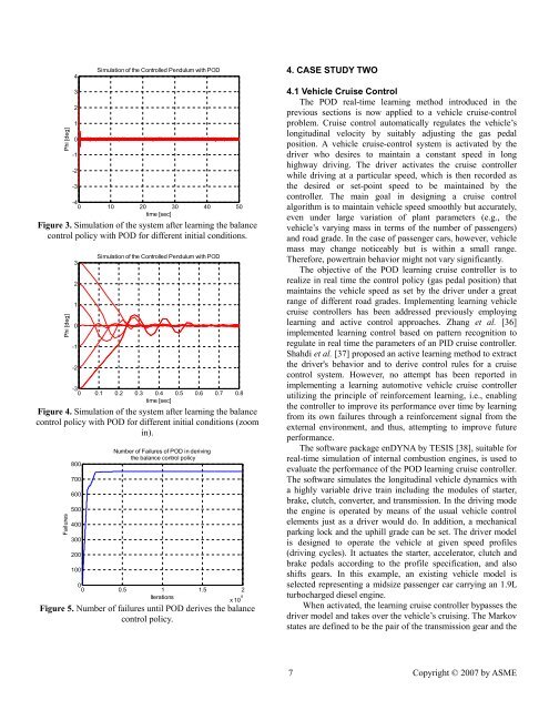
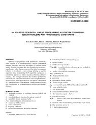
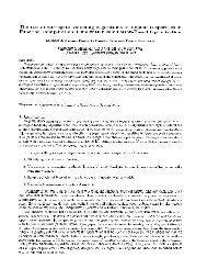
“neural-fuzzy BOXES” control system by neural networks andutilized reinforcement learning for the training. Jeen-Shing etal. [33] proposed a defuzzification method incorporating agenetic algorithm to learn the defuzzification factors. Mustaphaet al. [34] developed an actor-critic reinforcement learningalgorithm represented by two adaptive neural-fuzzy systems. Siet al. [35] proposed a generic on-line learning control systemsimilar to Anderson’s utilizing neural networks and evaluated itthrough its application to both a single and double cart-polebalancing problem. The system utilizes two neural networks,and employs the action- dependent heuristic dynamicprogramming to adapt the weights of the networks.In the implementation of the POD on the single invertedpendulum presented here, two major variations are considered:(a) a single look-up table-based representation is employed forthe controller to develop the mapping from the system’sMarkov states to optimal actions, and (b) two system’s statevariables are selected to represent the Markov state. The latterintroduces uncertainty and thus a conditional probabilitydistribution associating the state transitions with respect to theactions taken. Consequently, the POD method is evaluated inderiving the optimal policy (balance control policy) in asequential decision making problem under uncertainty.The governing equations, derived from the free bodydiagram of the system, shown in Figure 2, are:2( M + m) x + bx + mLϕcosϕ− mL ϕ sin ϕ = U , (19)2mLx cos ϕ+ ( I + mL ) ϕ+ mgL sinϕ= 0, (20)N secwhere M = 0.5 kg, m = 0.2 kg, b=0.1m2 mI = 0.006 kg m , g = 9.81 ,and L = 0.3 m.2secThe goal of the learning controller is to realize in real timethe force, U, of a fixed magnitude to be applied either to theright or the left direction so that the pendulum stands balancedwhen released from any angle, φ, between 3° and -3°. Thesystem is simulated by numerically solving the nonlineardifferential equations (19) and (20) employing the explicitRunge-Kutta method with a time step of τ =0.02 sec. Thesimulation is conducted by observing the system’s states andexecuting actions (control force U) with a sample rate T =0.02sec (50 Hz). This sample rate defines a sequence of decisionmakingepochs, T = 0,1, 2,..., M,M ∈N .The system is fully specified by four state variables: (a) theposition of the cart on the track, x()t ; (b) the cart velocity,x() t ; (c) the pendulum’s angle with respect to the verticalposition, ϕ () t ; and (d) the angular velocity, ϕ () t . However, toincorporate uncertainty, the Markov states are selected to beonly the pair of the pendulum’s angle and angular velocity,namely, the finite state space S, in Eq. (1) is defined asS = { s | s = ( ϕ, ϕ)}.(21)iiUN HN VMxxbxIϕ 2LϕmgN HFigure 2. Free body diagram of the system.IϕmI,Consequently, at state si∈S and executing a control forcevalue, U(s i ), the system will end up at state s j∈S with aconditional probably ps (j| si, Us (i)). The control force, U(s i ),selects values from the finite set A, defined asA = As (i) = [ − 3 N,3 N], where i= 1, 2,..., N, N=| S | . (22)The decision-making process occurs at each of a sequence ofepochs T = 0,1, 2,..., M,M ∈ N . At each decision epoch, thelearning controller observes the system’s state s i∈S , andexecutes a control force value U( si) ∈ A( si). At the nextdecision epoch, the system transits to another statesj∈S imposed by the conditional probabilitiesps (j| si, Us (i)), and receives a numerical reward (thependulum’s angle φ).The inverted pendulum is simulated repeatedly fordifferent initial angles, φ, between 3° and -3° utilizing the PODlearning method. The simulation lasts for 50 sec and eachcomplete simulation defines one iteration. If at any instantduring the simulation, the pendulum’s angle, φ, becomesgreater than 3° or less than -3°, this constitutes a failure,denoted by stating that there was one iteration associated with afailure. If, however, no failure occurs during the simulation,this is denoted by stating that there was one iteration associatedwith no failure.3.2 Simulation ResultsAfter completing the learning process, the controller employingthe POD learning method realizes the balance control policy ofthe pendulum, as illustrated in Figure 3. In some instances,however, the system’s response demonstrates some overshootsor delays during the transient period, shown in Figure 4. Thiscan be handled by a denser parameterization of the state-spaceor adding a penalty in long transient responses. The efficiencyof the POD learning method in deriving the optimal balancecontrol policy that stabilizes the system is illustrated in Figure5. It is noted that after POD realizes the optimal policy in 749failures and, afterwards, as the number of iterations continuesno further failures occur.N Vx6 Copyright © 2007 by ASME
Phi [deg]43210-1-2-3Simulation of the Controlled Pendulum with POD-40 10 20 30 40 50time [sec]Figure 3. Simulation of the system after learning the balancecontrol policy with POD for different initial conditions.Phi [deg]3210-1-2Simulation of the Controlled Pendulum with POD-30 0.1 0.2 0.3 0.4 0.5 0.6 0.7 0.8time [sec]Figure 4. Simulation of the system after learning the balancecontrol policy with POD for different initial conditions (zoomin).Failures800700600500400300200100Number of Failures of POD in derivingthe balance control policy00 0.5 1 1.5 2Iterationsx 10 4Figure 5. Number of failures until POD derives the balancecontrol policy.4. CASE STUDY TWO4.1 Vehicle Cruise ControlThe POD real-time learning method introduced in theprevious sections is now applied to a vehicle cruise-controlproblem. Cruise control automatically regulates the vehicle’slongitudinal velocity by suitably adjusting the gas pedalposition. A vehicle cruise-control system is activated by thedriver who desires to maintain a constant speed in longhighway driving. The driver activates the cruise controllerwhile driving at a particular speed, which is then recorded asthe desired or set-point speed to be maintained by thecontroller. The main goal in designing a cruise controlalgorithm is to maintain vehicle speed smoothly but accurately,even under large variation of plant parameters (e.g., thevehicle’s varying mass in terms of the number of passengers)and road grade. In the case of passenger cars, however, vehiclemass may change noticeably but is within a small range.Therefore, powertrain behavior might not vary significantly.The objective of the POD learning cruise controller is torealize in real time the control policy (gas pedal position) thatmaintains the vehicle speed as set by the driver under a greatrange of different road grades. Implementing learning vehiclecruise controllers has been addressed previously employinglearning and active control approaches. Zhang et al. [36]implemented learning control based on pattern recognition toregulate in real time the parameters of an PID cruise controller.Shahdi et al. [37] proposed an active learning method to extractthe driver's behavior and to derive control rules for a cruisecontrol system. However, no attempt has been reported inimplementing a learning automotive vehicle cruise controllerutilizing the principle of reinforcement learning, i.e., enablingthe controller to improve its performance over time by learningfrom its own failures through a reinforcement signal from theexternal environment, and thus, attempting to improve futureperformance.The software package enDYNA by TESIS [38], suitable forreal-time simulation of internal combustion engines, is used toevaluate the performance of the POD learning cruise controller.The software simulates the longitudinal vehicle dynamics witha highly variable drive train including the modules of starter,brake, clutch, converter, and transmission. In the driving modethe engine is operated by means of the usual vehicle controlelements just as a driver would do. In addition, a mechanicalparking lock and the uphill grade can be set. The driver modelis designed to operate the vehicle at given speed profiles(driving cycles). It actuates the starter, accelerator, clutch andbrake pedals according to the profile specification, and alsoshifts gears. In this example, an existing vehicle model isselected representing a midsize passenger car carrying an 1.9Lturbocharged diesel engine.When activated, the learning cruise controller bypasses thedriver model and takes over the vehicle’s cruising. The Markovstates are defined to be the pair of the transmission gear and the7 Copyright © 2007 by ASME
Page 1 and 2: Proceedings of IMECE072007 ASME Int
Page 3 and 4: which causes the system to perform
Page 8 and 9: difference between the desired and
Page 10: [15] Sutton, R. S., "Integrated Arc

A State-Space Representation Model and Learning Algorithm for ...

Create successful ePaper yourself

Delete template?

Save as template?