A State-Space Representation Model and Learning Algorithm for ...

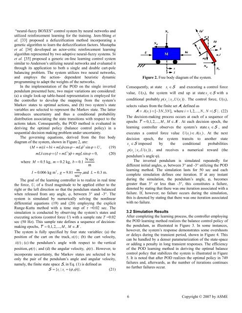
“neural-fuzzy BOXES” control system by neural networks andutilized reinforcement learning for the training. Jeen-Shing etal. [33] proposed a defuzzification method incorporating agenetic algorithm to learn the defuzzification factors. Mustaphaet al. [34] developed an actor-critic reinforcement learningalgorithm represented by two adaptive neural-fuzzy systems. Siet al. [35] proposed a generic on-line learning control systemsimilar to Anderson’s utilizing neural networks and evaluated itthrough its application to both a single and double cart-polebalancing problem. The system utilizes two neural networks,and employs the action- dependent heuristic dynamicprogramming to adapt the weights of the networks.In the implementation of the POD on the single invertedpendulum presented here, two major variations are considered:(a) a single look-up table-based representation is employed forthe controller to develop the mapping from the system’sMarkov states to optimal actions, and (b) two system’s statevariables are selected to represent the Markov state. The latterintroduces uncertainty and thus a conditional probabilitydistribution associating the state transitions with respect to theactions taken. Consequently, the POD method is evaluated inderiving the optimal policy (balance control policy) in asequential decision making problem under uncertainty.The governing equations, derived from the free bodydiagram of the system, shown in Figure 2, are:2( M + m) x + bx + mLϕcosϕ− mL ϕ sin ϕ = U , (19)2mLx cos ϕ+ ( I + mL ) ϕ+ mgL sinϕ= 0, (20)N secwhere M = 0.5 kg, m = 0.2 kg, b=0.1m2 mI = 0.006 kg m , g = 9.81 ,and L = 0.3 m.2secThe goal of the learning controller is to realize in real timethe force, U, of a fixed magnitude to be applied either to theright or the left direction so that the pendulum stands balancedwhen released from any angle, φ, between 3° and -3°. Thesystem is simulated by numerically solving the nonlineardifferential equations (19) and (20) employing the explicitRunge-Kutta method with a time step of τ =0.02 sec. Thesimulation is conducted by observing the system’s states andexecuting actions (control force U) with a sample rate T =0.02sec (50 Hz). This sample rate defines a sequence of decisionmakingepochs, T = 0,1, 2,..., M,M ∈N .The system is fully specified by four state variables: (a) theposition of the cart on the track, x()t ; (b) the cart velocity,x() t ; (c) the pendulum’s angle with respect to the verticalposition, ϕ () t ; and (d) the angular velocity, ϕ () t . However, toincorporate uncertainty, the Markov states are selected to beonly the pair of the pendulum’s angle and angular velocity,namely, the finite state space S, in Eq. (1) is defined asS = { s | s = ( ϕ, ϕ)}.(21)iiUN HN VMxxbxIϕ 2LϕmgN HFigure 2. Free body diagram of the system.IϕmI,Consequently, at state si∈S and executing a control forcevalue, U(s i ), the system will end up at state s j∈S with aconditional probably ps (j| si, Us (i)). The control force, U(s i ),selects values from the finite set A, defined asA = As (i) = [ − 3 N,3 N], where i= 1, 2,..., N, N=| S | . (22)The decision-making process occurs at each of a sequence ofepochs T = 0,1, 2,..., M,M ∈ N . At each decision epoch, thelearning controller observes the system’s state s i∈S , andexecutes a control force value U( si) ∈ A( si). At the nextdecision epoch, the system transits to another statesj∈S imposed by the conditional probabilitiesps (j| si, Us (i)), and receives a numerical reward (thependulum’s angle φ).The inverted pendulum is simulated repeatedly fordifferent initial angles, φ, between 3° and -3° utilizing the PODlearning method. The simulation lasts for 50 sec and eachcomplete simulation defines one iteration. If at any instantduring the simulation, the pendulum’s angle, φ, becomesgreater than 3° or less than -3°, this constitutes a failure,denoted by stating that there was one iteration associated with afailure. If, however, no failure occurs during the simulation,this is denoted by stating that there was one iteration associatedwith no failure.3.2 Simulation ResultsAfter completing the learning process, the controller employingthe POD learning method realizes the balance control policy ofthe pendulum, as illustrated in Figure 3. In some instances,however, the system’s response demonstrates some overshootsor delays during the transient period, shown in Figure 4. Thiscan be handled by a denser parameterization of the state-spaceor adding a penalty in long transient responses. The efficiencyof the POD learning method in deriving the optimal balancecontrol policy that stabilizes the system is illustrated in Figure5. It is noted that after POD realizes the optimal policy in 749failures and, afterwards, as the number of iterations continuesno further failures occur.N Vx6 Copyright © 2007 by ASME