Optimal Engine Design Using Nonlinear Programming and the ...

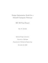
This is an unofficial copy of a technical report jointly published byFord Motor Co. Scientific Research Laboratories, Dearborn Michiganand the Department of Mechanical Engineering at the University o fMichigan, Ann Arbor, August 15 1991OPTIMAL ENGINE DESIGN USING NONLINEAR PROGRAMMINGAND THE ENGINE SYSTEM ASSESSMENT MODELbyTerrance C. Wagner (1)andPanos Y. Papalambros (2)A Sequential Quadratic Programming optimization algorithm was interfaced to the Engine SystemAssessment (ESA) model to determine the optimal combustion chamber geometry to maximize power. Both netpower and power per unit displacement were studied, together with packaging, fuel economy and knock limitingconstraints. Sensitivity of the optimal solution to changes in constraint parameters was also studied. Changes in thefuel economy and the displacement volume specifications affected the optimal design. It is shown that the problem ofoptimizing power is one of maximizing bore without exceeding the package constraint and/or degrading fuel economy.Also, to optimize net power subject to package constraints, the displacement volume should be treated as a variablesubject to package constraints and not specified a priori.Two algebraic models are developed first,based on ESA expressions; one for a flat head design and one for acompound valve head design. They are used with monotonicity analysis to determine a partial solution analytically.The analytical results and the numerical results with the ESA program gave identical solutions for the geometricdesign variables. Absolute values of brake power and specific fuel consumption differed because the algebraicexpressions contained incomplete friction models.While the optimal designs concluded from this work may be readily apparent to experienced engine engineers,the readily available sensitivity of the optimal design to changes in constraint parameters is not. Therein lies theutility of the described approach. The optimization algorithm, the interface, and relevant future work are alsodescribed.APPROVED: ______________________________________R.J. Tabaczynski, ManagerEngine Research Department______________________________________________________________________(1) Engine Research Department, Research Staff(2) Professor, Department of Mechanical Engineering and Applied Mechanics,1

The University of Michigan, Ann Arbor, MI.2

1. IntroductionEngine modeling activities at Ford have the long term goal of reducing productdevelopment time and cost and improving product value. By providing sufficiently accuratesimulations these models enable engineers to assess the effects of engine design variables on bothengine commodity objectives and, with the complementary use of the Corporate VehicleSimulation Program (CVSP), the effects on vehicle objectives. Sufficiently accurate models canbe used to seek optimal designs, but to date, the methods represent an arduous task for the user.An array of design variables is usually determined by the user and a batch file is built to run thegiven model with this array of inputs. The output is then regressed in terms of those variables andthe optimum sought by the user. (See for example, the use of Taguchi Design of Experimentstechniques by Kenney et.al. [1989].) This paper demonstrates the utility of incorporatingnumerical optimization methods into this process.Specific advantages result from such an approach. The reduction of workload in seekingthe optimum is the most obvious. With the appropriate interface of a model to an optimizationsoftware package the user can readily study design solutions by changing the set of designvariables, the design objective and constraints, and examining the effects of widening ornarrowing the constraint boundaries.In this report, optimization techniques are used in internal combustion engine design toobtain preliminary values for a set of combustion chamber design variables that maximize poweroutput per unit displacement volume while meeting specific fuel economy and packagingconstraints. Two types of mathematical optimization models are used: an explicit algebraic modelobtained by simplifying expressions found in the Engine System Assessment program [Belaire andTabaczynski, 1985] and an optimization model which uses the Engine System Assessmentprogram directly as a function generator. Two combustion chamber geometries are studied withthe algebraic model, a simple flat head design and a compound valve head design.The report is organized as follows. A brief review of the use of numerical optimizationtechniques (including applications to engine design) is provided. Next, the development of theexplicit algebraic models are presented followed by some analysis on boundedness and constraintactivity. Relevant features of the ESA model are described next. Computational results are thenpresented for both the algebraic models and the ESA program. Lastly, extensive parametricstudies are presented to show how changes in parameter values affect the optimal design.The work described here is preliminary. The advantages of extending these techniques tomore detailed models like the Engine Simulator (ENGSIM) and the Corporate Vehicle SimulationProgram (CVSP) should become apparent. ESA was selected as the first model because of its ease1

of use, its explicit algebraic expressions and its continued proliferation into the companyoperations.2. Optimization MethodsThe terms objective, constraint, variable, parameter, vector, and feasible domain haveexplicit definitions given below.The objective is the quantity to be optimized (minimized or maximized). It can be anexplicit algebraic function or it can be an output of another computer program .A (design)variable is any quantity allowed to vary during the search for the optimumobjective. At least the objective function or one of the constraints should depend on a variable;otherwise it is not relevant to the problem statement.A parameter is any quantity appearing in the problem statement which is fixed during theoptimization. For example, the values of the bounds appearing in the constraint set are parameters.A constraint bounds the set of variables in some way. Examples are: upper and lowerbounds on variables, equality relationships among variables, upper and lower bounds on explicitalgebraic expressions relating design variables or upper and lower bounds on outputs of a model.The set of variable values bounded by the set of constraints is called the feasible domain.A vector is simply a set of scalars. The set of variables is a vector; the set of equalityconstraints is a vector; the set of inequality constraints is a vector. Also recall from multivariablecalculus that the gradient of a scalar is a vector; and that the gradient of a vector is a matrix.2.1 Unconstrained OptimizationThe goal of optimization is to minimize or maximize a single function f, which depends onone or more independent variables. The value of those variables at that minimum or maximum andthe value of f is termed the optimal solution. The calculation of gradients in the design variablespace in search of a minimum is the essence of the algorithms of interest here. For acomprehensive, understandable introduction to optimization see Chapter 10 of Numerical Recipes- The Art of Scientific Computing, [Press, et.al.,1987].The classical statement of an unconstrained optimization problem is to minimize (ormaximize) a function f which depends upon a vector, x, of n variables where x = {x 1 ,x 2 , ......,x n ,} . The statement of the problem for x is:minimize f(x)x = {x 1 ,x 2 , ......, x n ,} ε R n (1)For a single variable problem, (x = {x}) recall from calculus that the first order necessarycondition for a minimum is df/dx = 0. Also recall that the value of d 2 f/dx 2 at this value of x2

sufficiently determines whether the function is a minimum or maximum; it is called the secondorder sufficiency condition . Similarly, for a function of n variables the first order necessarycondition is that the gradient of f(x) be equal to zero. That is:∂ f = 0∂x 1∇f(x) = ∂ f = 0 (2)∂x 2. .. .∂ f = 0∂x nThis results in a set of n equations that must be solved. Newton's method is a straightforwardalgorithm to solve such a set of equations. The following steps describe the algorithm .Step 1.Step 2.Pick a starting point (a guess of the solution) x 0 and set an iteration counterk = 0. (Superscript indicates iteration number).Calculate a step size, d k , to move in x whered k = -[D(∇f(x) ) k ] -1 (∇f(x) ) k (3)and D(∇f(x) )is the Jacobian of the gradient of f(x) and the Hessian of f(x).Step 3.Calculate a new value of x usingx k+1 = x k + d k (4)Step 4. If a convergence criteria is satisfied (e.g. || x k+1 - x k || ≤ ε) stop;otherwise increment k by one and go to 2.For quadratic functions, it can be shown that this method converges in one step from the startingpoint [Dennis et al., 1989].2.2 Constrained OptimizationMost design problems have many constraints imposed. For example, engine designproblems include geometric constraints on the engine package, and performance criteria constraintson the vehicle. The constraints can be in the form of an equality ( e.g., π (bore) 2 x (stroke) - 4(volume) = 0) or an inequality (e.g., (maximum piston speed) - 25m/sec ≤ 0). Each equalityconstraint equation is valued at 0 and is usually denoted by h. Similarly, inequalities are3

expressions set less than or equal to 0 and are denoted by g. Table I shows a formal statement of aconstrained minimization problem .Table 1. Example of Constrained Minimization Problemminimize f (x) (x 1 + 3x 2 +x 3 ) 2 + 4(x 1 -x 2 ) 2subject to:h1(x) = 0 1-x 1 - x 2 - x 3 = 0g1(x) ≤ 0 3 + x 13 - 4x 3 - 6x 2 ≤ 0g2(x) ≤ 0 -x 1 ≤ 0g3(x) ≤ 0 -x 2 ≤ 0g4(x) ≤ 0 -x 3 ≤ 0In shorthand the formal statement of this problem is:min f(x)subj. to : h(x) = 0 (5)g(x) ≤ 0where h(x) = {h 1 (x),h 2 (x),...,hm(x)} is a vector of equality constraints and g(x) ={g 1 (x),g 2 (x),...,g l (x )} is a vector of inequality constraints.2.2.1 The LagrangianA class of algorithms have been developed to solve this problem by minimizing a scalarfunction called the Lagrangian. It is a weighted sum of the objective function and the constraints.The weights are multipliers for each of the constraints. There are l multipliers for the equalityconstraints, λ = ( λ 1 , λ 2 ,... λ l) and m multipliers for the inequality constraints,µ = ( µ 1 , µ 2 ,... µ m ). Hence λ and µ are vectors. The Lagrangian is written asL = f(x) + ∑ l λ i h i (x) + ∑ m µ i g i (x) (6)and the optimization problem is stated asminimize L(x)subject to: µ ≥ 0 (7)λ ≠ 0.Formulation of the Lagrangian transforms a constrained minimization problem into an equivalentunconstrained minimization problem.4

2.2.2 The Karush-Kuhn-Tucker (KKT) ConditionsThe first order necessary condition for the minimization of the Lagrangian is that thegradient of the Lagrangian be equal to zero. (For proof see for example, Dennis et al. [1989]).∇ L = ∇f(x) + µ Τ ∇ h(x) + λ Τ ∇g(x) = 0 T (8)In addition, the following must hold.λ ≠ 0µ ≥ 0λ T h(x) = 0 Tµ T g(x) = 0 T (9)These are called the Karush-Kuhn-Tucker (KKT) conditions. and constitute the first ordernecessary conditions for the constrained optimization problem. One class of algorithms to solvethis problem is called Sequential Quadratic Programming (SQP) and is described briefly below.See Papalambros and Wilde [1988] or Luenberger [1984] for a more detailed discussion of SQPmethods.2.3 Sequential Quadratic Programming (SQP) MethodsSQP methods approximate the gradient of the Lagrangian with a first order Taylor'sexpansion. This is equivalent to approximating the Lagrangian as a quadratic function. Theconstraints are approximated with a linear approximation. An iterative algorithm to solve∇L(x) = 0results in solving a sequence of quadratic programming subproblems; hence the name SQP. Thesolution of the quadratic subproblem yields a step direction for the next iteration in the designspace. In addition, a line search algorithm is usually invoked to determine the best magnitude forthe direction found.2.4 Optimal Engine Design StudiesOptimization algorithms have been in use for some time to determine optimal controlschedules of air-fuel ratio, spark and exhaust gas recirculation as a function of speed and torque tomeet fuel and emissions requirements of the Environmental Protection Agency (EPA) driving cycle(see for example, Auiler et al. [1978]; Rishavy et al. [1977]). Physically based models of thecombustion process in internal combustion engines have been in use for over a decade (Blumberget al. [1980], Heywood [1980]; Kreiger [1980]; Reynolds [1980]) to predict the effects of relevantdesign changes in combustion chamber, valve/port interface, and valve timing (Davis andBorgnakke [1981], Davis et al. [1986, 1988]; Newman et al. [1989]). However, optimal designs5

are still sought primarily through arduous studies varying one variable at time. These studiesusually involve a series of hill-climbing (or descending) algorithms which are both computationallyexpensive and non-convergent from the optimization viewpoint [Kenney et al. 1989, Luenberger1984].Kenney et al. [1989] discuss the use of design of experiments techniques to specify theoperating conditions for a parametric study, and use the General Engine Simulator to optimize camevent timing for improving idle stability of a 5.8L gasoline engine. They used the same techniqueto optimize cam timing for wide open throttle performance using Ford’s one-dimensionalcompressible flow model of the manifold fluid dynamics (MANDY, see Chapman et al. [1982] formodel description). Upper and lower variable bounds were the only constraints in both problems.Assanis and Polishak [1989] used the model of Poulos and Heywood [1983] to predict optimalcam timing. They predicted and experimentally verified a 5% increase in peak torque. Woodard etal. [1988] formulated and solved a nonlinear programming problem using Campbell's model[1979] with a general conjugate gradient method to minimize fuel consumption at a single operatingcondition representing vehicle cruise. They varied combustion chamber geometry and valve timingand predicted a 20% reduction in fuel consumption over the existing design. A clever techniquefor accommodation of the discrete cam timing variables was also presented.The work described above was directed at improving existing designs using detailedmodels that numerically integrate the energy equation for a full thermodynamic Otto cycle. Thework here presents the preliminary engine design problem as a nonlinear programming problemusing a "lumped" thermodynamic model as expressed in the technical appendix for the EngineSystem Assessment program [Belaire and Tabaczynski, 1985] ; similar empiricisms can be foundin the open literature (see for example, Bishop [1964]; Taylor [1985]; Heywood [1988]).The utility of such a model is to obtain an expedient first order approximation to the optimalengine configuration and the sensitivity of the optimum to changes in problem parameters, suchas package size and structural or manufacturability design rules. Such analysis is essential toefficiently allocate resources for optimal camshaft, port, piston, and valvetrain design with modelsof appropriate detail. In addition, an identical strategy, with appropriate resources, can be appliedto the execution of more complex programs such as ENGSIM and CVSP.6

inducted into the combustion chamber. The thermal efficiency accounts for the thermodynamicsassociated with the Otto cycle.Table 2. Nomenclature for Engine ModelAf air/fuel ratiob cylinder bore, mmBKW brake power, kWBMEP brake mean effective pressure, kPacr compression ratioCs port discharge coefficientdE exhaust valve diameter, mmdI intake valve diameter, mmEGR exhaust gas recirculation, percentFMEP friction mean effective pressure, barsh compound valve chamber deck height, mmH distance dome penetrates head, mmIMEP indicated mean effective pressure, kPaisfc indicated specific fuel consumption, g/kwhMAP manifold absolute pressure, kPaNc number of cylindersNv number of valvesQ lower heating value of fuel, kJ/kgr radius of compound valve chamber curvature, mms stroke of piston, mmSv surface to volume ratio, mm -1V, v displacement volume, mm 3vc clearance volume, mm 3vd dome volume, mm 3Vp mean piston speed, m/minw revolutions per minute at peak power , x 10 -3Zb RPM factor in volumetric efficiencyZn Mach Index of port/chamber designγη vratio of specific heats of in-cylinder gasesvolumetric efficiencyη vb base volumetric efficiencyη t thermal efficiencyη tad adiabatic thermal efficiencyη tw thermal efficiency at representative part loadpoint (1500 rpm, Af = 14.6)ρ density of inlet charge, kg/m 3φ equivalence ratio2

The volumetric efficiency can be expressed asη v = η vb (1 + Z b2 )/(1 + Zn 2 ) (13)where η vb is the base volumetric efficiency, Z b is the RPM factor in volumetric efficiency, and Z nis the Mach Index of port/chamber design. The base volumetric efficiency for a "best-in-class"engine may be expressed empirically with a curve-fitting formula in terms of RPM at peak power,w, as follows:η vb = 1.067 - 0.038 e w-5.25 for w > 5.25η vb = 0.637 + 0.13w - 0.014w 2 + 0.00066w 3 for w ≤ 5.25 (14)Also empirically [Taylor 1985], for a speed of sound of 353 m/sec we setZ b = 7.72 (10 -2 )w (15)Z n = 9.428 (10 -5 ) ws(b/d I ) 2 /C s (16)where s is the piston stroke, b is the cylinder bore, d I is the intake valve diameter and C s is the portdischarge coefficient, a parameter characterizing the flow losses of a particulardesign.manifold and portbHead FacedIdEh = s/(cr - 1)Position atTop Dead CentersFigure 1. Schematic of geometry for flat head designThe thermal efficiency is expressed asη t = η tad - .083 S v (1.500/w) 0.5 (17)where η tad is the adiabatic thermal efficiency given byη tad = 0.9 (1-c r(1-γ) )(1.18 - 0.225φ) for φ < 1= 0.9 (1-c r(1-γ) )(1.655 - 0.7φ) for φ > 1 (18)and the S v term accounts for heat transfer effects due to surface/volume ration of the chamber.Here c r is the compression ratio, γ is the ratio of specific heats of the in-cylinder gases, and φ isthe equivalence ratio that accommodates air-fuel ratios different from stoichiometric. In the optimal3

design model stoichiometry will be assumed, so that φ = 1 and the two expressions in Eq.(18) willgive the same result. The thermal efficiency for an ideal Otto cycle would be (1-c r(1-γ) ). The 0.9multiplier in the formulas accounts empirically for the fact that the heat release occurs over finitetime, rather than instantaneously as in an ideal cycle, and it is assumed valid for displacements onthe order of 400 to 600 cc/cylinder and bore-to-stroke ratios between 0.7 and 1.3 [Belaire andTabaczynski, 1985]. Heat transfer is accounted for by the product of the surface-to-volume ratioof the cylinder, S v , and an RPM correction factor. The surface-to-volume ratio is expressed asS v = [(0.83) (12s + (cr - 1)(6b + 4s))]/[bs (3 + (cr - 1))] (19)for a reference speed of 1500 rpm and 4.14 bar of IMEP.Finally the FMEP is derived with the simple assumption that the operating point of interestwill be near wide open throttle, the point used for engine power tests, and that engine accessoriesare ignored. Under these conditions pumping losses are small and ignored. The primary factorsaffecting engine friction are compression ratio and engine speed. An expression to reflect this isFMEP = (4.826)(cr - 9.2) + (7.97 + 0.253Vp + 9.7(10 -6 )Vp 2 ) (20)where Vp is the mean piston speed. More complete expressions (e.g., Bishop 1964, Patton etal. 1989) were not employed in order to keep the monotonicity analysis of the algabraic modeltractable.The constraints included are packaging and efficiency constraints. The packagingconstraints are as follows. We chose the maximum length of the engine block to be L1 = 400 mm.This limit constrains the bore using the practical design rule that the distance separating thecylinders should be greater than a certain percentage of the bore dimension. Therefore, for an inlineengineK1Ncb ≤ L1 (21)where the constant K1 = 1.2 for a cylinder separation of at least 20% of the bore, and Nc is thenumber of cylinders in the block. Similarly, engine height limit of L2 = 200 mm constrains thestroke:K2s ≤ L2 (22)where K2 = 2. For a flat cylinder head, geometric and structural constraints require the intake andexhaust valve diameters to satisfy the relationshipdI + dE ≤ K3b (23)where K3 = 0.82, and the ratio of exhaust valve to inlet valve diameter is restricted asK4 ≤ dE/dI ≤ K5 (24)4

where K4 = 0.83 and K5 = 0.87. Finally, the displacement volume is a given parameter related todesign variables byV = πNcb 2 s/4 (25)We now examine efficiency-related constraints. To preclude significant flow losses due tocompressibility of the air-fuel charge during induction the Mach Index of port/chamber designmust be less than K6 = 0.6 [Taylor 1985 ]:Z n = 9.428 (10 -5 ) ws(b/d I ) 2 /C s ≤ K6 (26)Knock-limited compression ratio for 98 octane fuel can be represented by [Heywood 1988]:c r ≤ 13.2 - 0.045b (27)The rated RPM at which maximum power occurs should not exceed the limits of the torqueconverter in conventional automatic transmissions, K7 = 6.5 (x1000 rpm). Therefore,w ≤ K7. (28)Fuel economy at part load (1500 rpm , A f = 14.6) is a representative restriction on overall fueleconomy. Therefore, a constraint is imposed on the indicated specific fuel consumption, isfc, atthis part load:isfc = 3.6 (10 6 ) (η tw Q) -1 ≤ K8 (29)where η tw is the part-load thermal efficiency and K8 = 230.5 g/kWh.In order to assign parameter values, we select specifications for a 1.86L four- cylinderengine. For this engine configuration maximizing power density is important. The followingvalues are then used for the parameters.ρ = 1.225 kg/m 3 γ = 1.33 V = 1.859 (10 6) mm 3Q = 43958 kJ/kg Nc = 4 Cs = 0.44 (30)Af = 14.6The ratio of specific heats is computed from the expressionγ = 1.33 + 0.01 (EGR/30) (31)with zero recirculation assumed, so γ = 1.33.The expression for thermal efficiency (and hence also fuel consumption) uses a singlemultiplier to account for time losses related to flame propagation rates. The value of 0.9 in Eq.(18)is considered valid within the limited range of bore-to-stroke ratios of0.7 ≤ b/s ≤ 1.3 (33)Outside this range, the geometry significantly affects flame propagation. Presumably, adependence of the multiplier on bore-to-stroke ratio could be developed and used. This was notdone in the present model, so Eq. (33) is treated as a set constraint, not included explicitly in themodel but checked after results have been obtained. Also note that the treatment of Cs as a5

parameter implies Cs is independent of valve size. This assumption requires scrutiny if Equation(23) is not satisfied as a strict equality.The model is now assembled after elimination of the stroke variable using the equalityconstraint on displacement volume, Equation (25), and is cast into a standard NLP form, theobjective being to minimize negative specific power (BKW/V).whereMODEL A (34)Minimize f = K0(FMEP - (ρQ/Af) η t η v ) w (in kW/liter)η v = η vb [1 + 5.96x10 -3 w 2 ]/[1 + [(9.428x10 -5 (4V/πNcCs)(w/d I2 )] 2 ]η vb = 1.067 - 0.038e w-5.25 for w > 5.25= 0.637 + 0.13 w - 0.014 w 2 + 0.00066w 3 for w ≤ 5.25η t = η tad - S v (1.5/w) 0.5η tad = 0.8595 (1- c r- 0.33 )S v = (0.83) [(8 + 4cr) + 1.5(cr - 1)(πNc/V)b 3 ]/[(2+ cr)b]FMEP = (4.826)(cr - 9.2) + (7.97 + 0.253 Vp + 9.7(10 -6 )Vp 2 )Vp = (8V/πNc)wb -2subject tog1 = K1Ncb - L1 ≤ 0min bore wall thicknessg2 = (4K2V/πNcL2) 1/2 - b ≤ 0max engine heightg3 = dI + dE - K3b ≤ 0valve geometry and structureg4 = K4 dI - dE ≤ 0min valve diameter ratiog5 = dE - K5 dI ≤ 0max valve diameter ratiog6 = (9.428)(10 -5 )(4V/πNc)(w/d I2 ) - K 6Cs ≤ 0 max port/chamber Mach Indexg7 = cr - 13.2 + 0.045 b ≤ 0knock-limited compression ratiog8 = w - K7 ≤ 0max torque converter rpmg9 = 3.6 (10 6 ) - K8Qη tw ≤ 0min fuel economy at part loadwhere η tw = 0.8595 (1- c r- 0.33 ) - SvThis concludes the initial modeling effort for the flat head design problem. Note that there are fivedesign variables, b, dI, dE, cr, and w. There are nine inequality and no equality constraints, as allequalities that appear in Model A are simple definitions of intermediate quantitiesappearing in the inequalities. Significant parameters, for which numerical values were given inEquation (30), are maintained in Model A with their symbols for easy reference in subsequentparametric post-optimality studies. Parameter values dictated by current practice or given design6

specifications are indicated by the Ki (i = 1,..., 12) and Li ( i = 1, 2) coefficients and summarizedin Table 3.3.1.2 Model B - Compound Valve Head Chamber GeometryThe geometry for the compound valve head design is shown in Figure 2. Accounting forthis new geometry will change Model A presented above with the addition of new design variablesand constraints. The new variables are the displacement volume v (considered a parameter inModel A), the deck height h, and the radius of curvature r. As displacement is now a variable,the objective function is selected to be brake power rather than specific brake power. Arelationship between clearance volume vc, displacement volume v, and compression ratio isimposed by the definition of the compression ratio:cr = (v/Nc + vc)/vc (35)dEHhead facerFigure 2. Schematic for compound valve designwhereThe clearance volume is the sum of deck volume and dome volume vd.vc = πhb 2 /4 + vd (36)vd = (1/3)π[(r 2 - b 2 /4) 1.5 - (r 2 - dI 2 /4) 1.5 - (r 2 - dE 2 /4) 1.5 ]- πr 2 [(r 2 - b 2 /4) 0.5 - (r 2 - dI 2 /4) 0.5 - (r 2 - dE 2 /4) 0.5 ] - (2/3)π r 3 (37)7

A typical design specification on the deck height ish = K11b (38)where K11 = 1/64. A minimum distance of K12b must separate the two valves (Taylor 1985),where K12 = 0.125. Geometrically this can be approximated by setting(dI 2 - H 2 ) 0.5 + (dE 2 - H 2 ) 0.5 ≤ ( 1- K12) b (39)where H is the distance the dome penetrates the head (Figure 2) and is defined asH = r - (r 2 - b 2 /4) 0.5 (40)In standard NLP form the problem of maximizing power for the compound valve head geometrybecomeswhereMODEL B (41)Minimize f = K0(FMEP - (ρQ/Af) η t η v ) wvη v = η vb [1 + 5.96x10 -3 w 2 ]/[1 + [(9.428x10 -5 (4v/πNcNvCs)(w/d I2 )] 2 ]η vb = 1.067 - 0.038e w-5.25 for w > 5.25= 0.637 + 0.13 w - 0.014 w 2 + 0.00066w 3 for w ≤ 5.25η t = η tad - S v (1.5/w) 0.5η tad = 0.9 (1- c r- 0.33) )(1.18 - 0.225φ) for φ < 1= 0.9 (1- c r- 0.33 )(1.655 - 0.7φ) for φ > 1S v = (0.83) [(8 + 4cr) + 1.5(cr - 1)(πNc/v)b 3 ]/[(2+ cr)b]FMEP = (4.826)(cr - 9.2) + (7.97 + 0.253 Vp + 9.7(10 -6 )Vp 2 )Vp = (8v/πNc)wb -2subject to:h1 = cr - (v/Nc + vc)/vc = 0compression ratio definitionwhere vc = πhb 2 /4 + vdvd = (1/3)π[(r 2 - b 2 /4) 1.5 - (r 2 - dI 2 /4) 1.5 - (r 2 - dE 2 /4) 1.5 ]- πr 2 [(r 2 - b 2 /4) 0.5 - (r 2 - dI 2 /4) 0.5 - (r 2 - dE 2 /4) 0.5 ] - (2/3)π r 3h2 = h - K11b = 0deck height specificationg1 = K1Ncb - L1 ≤ 0min bore wall thicknessg2 = (4K2v/πNcL2) 1/2 - b ≤ 0max engine heightg3 = (dI 2 - H 2 ) 0.5 + (dE 2 - H 2 ) 0.5 - K3cb ≤ 0 min valve distancewhere H = r - (r 2 - b 2 /4) 0.5g4 = K4 dI - dE ≤ 0min valve diameter ratiog5 = dE - K5 dI ≤ 0max valve diameter ratiog6 = (9.428)(10 -5 )(4v/πNc)(w/d I2 ) - K 6Cs ≤ 0 max port/chamber Mach Index8

g7 = cr - 13.2 + 0.045 b ≤ 0 knock-limited compression ratiog8 = w - K7 ≤ 0max torque converter rpmg9 = 3.6 (10 6 ) - K8Qη tw ≤ 0min fuel economy at part loadwhere η tw = 0.8595 (1- c r- 0.33 ) - Svg10 = v - K9 ≤ 0g11 = - v + K10 ≤ 0The empirical parameters have the same values as in Model A in addition to K3c = 1 - K12 =0.875, K9 = 1.6(10 6 ), K10 = 2.3(10 6 ). There are two equality constraints (h 1 and h 2 ) added tothis model. In principle, one design variable can be eliminated for each equality (e.g. cr, and h).However, this creates an algebraic nightmare for the other contraints, so no model reduction willbe attempted using the equality constraints. Constraint g 3 has been rewritten and two additionalinequalities, g 10 and g 11 , have been added to provide upper and lower bounds on the displacementvolume.Table 3. Current Practice or Design Specification ParametersPARAMETERVALUESPECIFICATIONK0K1K2K3K4K5K6K7K8K9K10K11K12L1L21/1201.220.820.830.890.66.5230.5 g/kWh2.3 (106)mm31.6 (106)mm31/640.125400 mm200 mmunit conversion, 4 stroke enginecylinder separation as % of boreengine height as a multiple of strokevalve spacing as % of bore (flat head)lower bound on valve ratioupper bound on valve ratioupper bound on Mach Indexupper bound on rpmupper bound on isfcupper bound on displacement volumelower bound on displacement volumebore fraction specification for deck heightbore fraction specification for valve distanceupper bound on engine block lengthupper bound on engine block height9

3.2 Monotonicity AnalysisIn many design models, the objective and constraint functions are monotonic with respectto the design variables. A continous differentiable function f(x) is monotonically increasing withrespect to (wrt) a design variable x i , if ∂f/∂xi > 0; it is monotonically decreasing wrt a designvariable x i , if ∂f/∂xi < 0. Under either condition, we say that f is coordinate-wise monotonic wrtxi, or that xi is a monotonic variable in f. Monotonicity analysis is a model analysis methodologythat checks whether a model is properly bounded and identifies active constraints when possible.Active inequality constraints must be satisfied as strict equalities at the optimum and theycorrespond to critical design requirements. See Papalambros and Wilde (1988) for further details.We start monotonicity analysis of Model A by identifying any monotonicities in the modelfunctions. Examining the model we observe the following.FMEP = FMEP(cr , Vp + (w + , b - )) = FMEP(cr, w + , b - )η t = η t (cr + , S - v (c r, b + )) = η t (cr, b - ) (42)η v = η v (w, d I+ )In Equation (42) the right hand side shows how the functions on the left depend on the designvariables. A superscript sign indicates the type of monotonicity that may exist, positive (ornegative) indicating that the function is increasing (or decreasing) wrt to that variable; no signindicates that the variable has undetermined monotonicity. All monotonicities above are easy toverify except that wrt b. Although the proof is omitted here, it is worth noting that it is a regionalmonotonicity, namely, valid only for the range of design variable values within the feasibledomain.The monotonicities of Model A can be now presented as follows.MODEL A1 (43)min f(cr, w, b, d - I ) = K0w [FMEP(cr, w + , b - ) - P 0 η t (cr, b - ) η v (w, d + I )]subject tog1(b + ) = b - P1 ≤ 0g2(b - ) = P2 - b ≤ 0g3(b - , dE + , d + I ) = dI + dE - K3 b ≤ 0g4(dE - , d + I ) = K4 dI - dE ≤ 0g5(dE + , d - I ) = dE - K5 dI ≤ 0g6(w + , d - I ) = P3 w - d I2 ≤ 0min bore wall thicknessmax engine heightvalve geometry and structuremin valve diameter ratiomax valve diameter ratiomax port/chamber Mach Index10

g7(cr + , b + ) = cr - 13.2 + 0.045 b ≤ 0knock-limited compression ratiog8(w + ) = w - K7 ≤ 0max torque converter rpmg9(cr, b + ) = P 4 - 0.8595(1- c r- 0.33 ) + Sv (cr, b + ) ≤ 0 min fuel economy at part loadNote that in this new model all known monotonicities are indicated and several parametric relationsPi have been introduced to simplify the presentation of the model. These are given in Table 4, thenumerical values corresponding to parameter values for the base case. We now proceed withrepresenting this information in a monotonicity table, as shown in Table 5.Table 4. Parametric Functions for Model AP 0 = ρQ/Af = 3688 kPaP 1 = L1/K1Nc = 83.33 mmP 2 = (4K2V/πNcL2) 1/2 = 76.90 mmP 3 = 9.428x10 -5 (4V/πNc)/(K6Cs) = 215.5 mm 2 secP 4 = 3.6(10 6 )/K8Q = .3412Table 5. Monotonicity Table for Model A1cr w b dE d If U U U -g1 +g2 -g3 - + +g4 - +g5 + -g6 + -g7 + -g8 +g9 U +11

In the monotonicity table the columns are the design variables and the rows are theobjective and constraint functions, the entries in the table being the monotonicities of each functionwith respect to each variable. Positive (negative) sign indicates increasing (decreasing) function, Uindicates undetermined or unknown monotonicity. An empty entry indicates that the function doesnot depend on the respective variable, so the table acts also as an incidence table.The Monotonicity Principles can be more readily applied using the monotonicity table.These principles state the following (Papalambros and Wilde 1988):First Monotonicity Principle (MP1): In a well-constrained objective function every increasing(decreasing) variable is bounded below (above) by at least one active constraint.Second Monotonicity Principle(MP2): Every monotonic variable not occurring in a wellconstrainedobjective function is either irrelevant and can be deleted from the problem together withall constraints in which it occurs, or is relevant and bounded by two active constraints, one fromabove and one from below.Based on these principles and Table 5 the following conclusions are reached. By MP1 wrtdI at least one of g3 or g4 must be active. We examine these two cases. (i) If g3 is active, then byMP2 wrt dE g4 must be active as well. (ii) If g4 is active, then by MP2 wrt dE g3 and/or g5 mustbe active. But g5 and g4 cannot be simultaneously active because they represent upper and lowerbounds on the same quantity. Therefore in case (ii) g4 must be active also. We see that in eithercase, both g3 and g4 must be active at the optimum. This is a necessary optimality condition thatmust be satisfied by any subsequent numerical results. Solving for dE and dI in terms of theoptimal value b * (asterisk denotes optimal value) we getdE * = b * K3K4/(1+K4)dI * = b * K3/(1+K4) (44)a solution that is acceptable provided K4 ≤ K5. Note that g5 is then inactive. Using the second ofEquation (44) to eliminate dI from the objective and remaining constraints Model A1 is nowreduced toMODEL A2 (45)min f(cr, w, b) = K0w [FMEP(cr, w + , b - ) - P 0 η t (cr, b - ) η v (w, b + )]subject tog1(b + ) = b - P1 ≤ 0g2(b - ) = P2 - b ≤ 0g6(w + , b - ) = P 3 w - [K3/(1+K4)] 2 b 2 ≤ 0g7(cr + , b + ) = cr - 13.2 + 0.045 b ≤ 0min bore wall thicknessmax engine heightmax port/chamber Mach Indexknock-limited compression ratio12

g8(w + ) = w - K7 ≤ 0max torque converter rpmg9(cr, b + ) = P 4 - 0.8595(1- c r- 0.33 ) + Sv (cr, b + ) ≤ 0min fuel economy at part loadwhere asterisks are dropped for convenience. There are only three design variables left and at mostthree constraints from the six in Model A2 can be active.We proceed with monotonicity analysis for Model B. We now haveFMEP = FMEP(cr , Vp + (w + , b - , v + )) = FMEP(cr, w + , b - , v + )η t = η t (cr + , S - v (c r, b + , v - )) = η t (cr, b - , v + ) (46)η v = η v (w, d + I , v - )v d = v d (b, d - I , dE - , r)The algebraic expression for v d in Equation (37) is not easy to use for proving the monotonicitieswrt d I and d E indicated above, but the geometry in Figure 2 shows that this is evidently the case.Eliminating variable h and constraint h2 we getMODEL B1 (47)min f(cr, w, b, d - I , v) = K 0wv [FMEP(cr, w + , b - , v + )- P 0 η t (cr, b - , v + ) η v (w, d + I , v - )]subject toh1(cr + , v - , vc - ) = - 1 + cr - (v /Ncvc) = 0 head geometrywhere vc = πK11b 3 /4 + vd(b, d - I , dE - , r)g1(b + ) = b - P1 ≤ 0min bore wall thicknessg2(b - , v + ) = P2C v 1/2 - b ≤ 0max engine heightg3(b, dE + , d + I , r) ≤ 0valve geometry and structureg4(dE - , d + I ) = K4 dI - dE ≤ 0min valve diameter ratiog5(dE + , d - I ) = dE - K5 dI ≤ 0max valve diameter ratiog6(w + , d - I , v + ) = P3C wv - d I2 ≤ 0max port/chamber Mach Indexg7(cr + , b + ) = cr - 13.2 + 0.045 b ≤ 0knock-limited compression ratiog8(w + ) = w - K7 ≤ 0max torque converter rpmg9(cr,b + ,v + )=P 4 - 0.8595(1- c r- 0.33 )+Sv (cr,b + ,v + ) ≤0min fuel economy at part load13

g10(v + ) ≤ 0g11(v - ) ≤ 0where the revised parametric functions areP 2C = (4K2/πNcL2) 1/2 P 3C = (9.428)(10 -5 )(4/πNc)/ (K6Cs). (48)Consider the implicit function h1(cr + , v - , b, d + I , dE + , r) = 0 defined by the equalityconstraint. If we use it to solve implicitly for d E we get d E = φ1(cr - , v + , b, d - I , r) based on theimplicit function theorem (Papalambros and Wilde 1988). Eliminating d E implicitly from Model B1we get the same model functions except that h1 is not present and g3, g4, g5 are replaced byg3'(b, d I , cr + , v - , r) ≤ 0g4'(d + I , c r + , v - , b, r) ≤ 0g5'(d - I , c r - , v + , b, r) ≤ 0 (49)By MP1 wrt d I at least one of g3' or g4' must be active, while by MP2 wrt r at least two of theabove three constraints must be active. Since g4' and g5' cannot be simultaneously active g3 isdefinitely active, but it cannot be concluded at this point that both g3 and g4 must be active as in thecase for flat heads. However, the problem has now one less variable and one less constraint. Thiscompletes the model analysis and the analytical results will be highlighted in the context of thenumerical results.3.3 The Optimizer NLPQL (NCONF).The NLPQL algorithm (Schittkowski, 1986) is available as a subroutine in the InternationalMathematical and Statistical Library (IMSL) [IMSL 1991] under the names NCONF andNCONG. It has been designed to solve the general nonlinear programming problem :min f(x)subject to: g j (x) = 0j=1,...,m eg j (x) ≥ 0 j=m e +1, ...., m (50)x l ≤ x ≤ x uNote the change in notation from Section 2 for the name of the equality constraint set and for thesign on the inequality constraint set. Also, note that variable bounds are specified separately fromthe constraint set. These changes are noted only to be consistent with the reference manuals on thealgorithm.It is assumed that all problem functions are continuously differentiable. The NLPQLalgorithm realizes a sequential quadratic programming method, also called recursive quadratic14

programming, constrained variable metric, or the algorithm of Powell [1978]. In each iteration aquadratic programming subproblem is formulated by linearizing the constraints and approximatingthe corresponding Lagrange function quadratically. A new iterate is calculated then by minimizinga so-called merit or penalty function along the search direction obtained from the subproblem. TheHessian matrix of the Lagrange function is approximated by the Broyden-Fletcher-Goldfarb-Shanno (BFGS) method. (See Papalambros and Wilde, [1988] p. 340 for a description of theBFGS method.)The main program that calls NCONF must contain an array of design variables, upper andlower bounds on those variables, and subroutines NLFUNC and NLGRAD. NLFUNC calculatesand returns the values of objective function and constraints at given variable values. NLGRADcalculates the gradient of the objective function and constraints with respect to the design variablesusing a forward difference approximation of the partial derivative. NLGRAD calls NLFUNC forthe forward difference calculation. Subroutines that calculate the gradient using other methods(including the analytical derivative if available) can be used in place of NLGRAD.3.4 Engine System Assessment ModelThe Engine System Assessment (ESA) program contains more comprehensive expressionsthan the analytical models given above. For example, it implements the friction model given byPatton et al. [1989]. Input engine geometry is described by 72 quantities, ten of which havecontinuous values; the remaining values are discrete and reflect specific design configurations.Examples of discrete-valued quantities are the number of cylinders, number of piston rings, andmultipliers that reflect specific component types such as a roller finger follower valvetrain. Outputsinclude a measure of WOT performance (volumetric efficiency or torque) as a function of enginespeed, analogous to the base volumetric efficiency curve in the analytical model, as well as theother engine performance quantities used in the analytical models above.3.5 The ESA-NLPQL InterfaceCoupling ESA and NCONF requires a means to pass variable values to ESA, call ESAfrom NCONF, and access ESA output. Three keys to the coupling are the ability to run ESA witha batch file, a 400 element array in ESA that contains all input and output data, and the use of asingle file called the problem definition file ('prob.def'). Appendix A shows the file contents withdescriptions. Figure 3 shows a schematic of the interface and data flow through the varioussubroutines. The main program performs three functions: it reads the problem definition file usinga subroutine called LOADPROB; it initializes the variables and sets bounds based on the contentsof 'prob.def'; and it invokes the optimizer subroutine NCONF once. NCONF invokes calls toNLFUNC to perform function evaluations and gradient evaluations. NCONF is the onlysubroutine that invokes ESA. This is accomplished by calling WRITE_INPUT to build a batch15

file to run ESA with the appropriate variable values; invoking a shell script to run ESA; and thenreading the contents of the 400 element array stored in 'dump.tmp'. The objective function andconstraints are evaluated with the relevant contents of the array.The design optimization model that uses ESA as the underlying analysis model is identicalto Model A with several exceptions. ESA serves now as an implicit function generator for theNLPQL optimizer. ESA is capable of providing peak power and RPM of peak power as output.This feature is exploited to minimize computational time during optimization iterations. Thevariable w (RPM) still appears in constraint g8 but only as an implicit function of the other fourdesign variables.Process invoked by shell script 'RUN_ESA'Batch filegeometry file namevariable changesflagsmanifold file nameESA'dump.tmp'(0,0)(20,20)MAINCALL LOADPROBInitialize bounds on variablesCALL NCONFNLFUNCCALL WRITE_INPUTInvoke script 'RUN_ESA'CALL READ_DUMPAssign objective and constraintsGRADIncrement variablesCALL NLFUNCLOADPROBOpen and read prob.defprob.defText Key- Description of actions- SUBROUTINE NAME- SUBROUTINE CALLWRITE_INPUTOpen 'in.tmp'Write file names, variables, flagsto in.tmpClose 'in.tmp'READ_DUMPOpen dump.tmpRead file into B arrayFigure 3. Schematic of ESA/NCONF interface.16

The problem statement presented to the optimizer is as follows:MODEL C (51)Minimize BKW/V = f1esa(b, dI, dE, cr; Af = 13.5, MAP = 99.63 kPa) (in kW/liter)subject tog1 = K1Ncb - L1 ≤ 0min bore wall thicknessg2 = (4K2V/πNcL2) 1/2 - b ≤ 0max engine heightg3 = dI + dE - K3b ≤ 0valve geometry and structureg4 = K4 dI - dE ≤ 0min valve diameter ratiog5 = dE - K5 dI ≤ 0max valve diameter ratiog6 = (9.428)(10 -5 )(4V/πNc)(w/d I2 ) - K 6Cs ≤ 0 max port/chamber Mach Indexg7 = cr - 13.2 + 0.045 b ≤ 0knock-limited compression ratiog8 = w esa (f1esa) - K7 ≤ 0max torque converter rpmg9 = (isfc) esa - K8 ≤ 0min fuel economy at part loadwhere(isfc) esa = f2esa(cr, b; Af = 14.6, BMEP = 262 kPa, RPM = 1500, EGR = 0% )The implicit function f1esa is a subroutine call that builds the ESA input files, invokes the ESAprogram at WOT conditions, and extracts the peak power density and the w at peak power from theavailable output. The implicit function f2esa is a subroutine call similar to f1esa that runs tthe ESAprogram at the part throttle condition and extracts the specific fuel consumption from the outputs.The variables in this functions and parameter value settings used are indicated in the model above.Note that ESA is called twice for each function call made by NLPQL.4. Computational Results and Parametric StudiesSubroutine NLPQL was used to solve Models A1, B1, and C numerically. Post-optimalparametric studies were performed to examine the sensitivity of the optimal solution with respect tosome key parameter values. Only some parametric results are presented below. Many differentcombinations of parameters can be examined, as long as the model validity assumptions are notviolated.Note that as NLPQL is capable of identifying only local solutions that satisfy the Karush-Kuhn-Tucker (KKT) first-order optimality conditions, it is possible that the solutions indicated aresaddlepoints rather than minima. However, the preceding model analysis that led to constraintactivity identification is a strong safeguard against this possibility.17

Iteration HistoryPredicted Brake Power( kW/liter)6056524801020SQP Iteration Number30f(kW/l)Bore/10, Compession Ratio,and RPM/1000 at Peak Power1098765401020SQP Iteration Number30crwb/1040Valve SizesdI, dE (mm)36dIdE3201020SQP Iteration Number30Figure 4. Search History of Optimization Algorithm Using Algebraic Model ofFlat Head Chamber (Model A1).18

4.1 Optimal Designs: Models A1, B1, and CResults for the "base case" of parameter values indicated in Tables 3 and 4 are presentedfirst. For flat head geometry Table 6 shows initial and final (optimal) values obtained by NLPQLafter twenty iterations. The iteration history is shown in Figure 4, as a typical example of thesearch pursued by the optimizer. Note that an SQP method will obtain intermediate infeasibleresults as part of its strategy.Table 6. Flat Head Geometry ResultsPowerDensityf (kW/l)Boreb (mm)IntakeValveDiameterdI (mm)ExhaustValveDiameterdE (mm)CompressionRatiocrRPMw*1000Starting Point 50.02 82.0 39.0 34.0 8.42 5000Final Point 60.7 83.3 40.5 33.6 9.45 6230Some observations on these results are as follows. At the initial design the value of RPMis not that of peak power and the value of cr is not the knock-limited compression ratio. The activeconstraints for the final design are the upper bound on bore wall thickness g1, the geometricrelationship between valves and bore g3, the minimum valve diameter ratio g4, and the knocklimitedcompression ratio g7. Activities for g3 and g4 were proven by monotonicity analysis. Forthe initial geometry, w = 6.13 (6130 rpm) and f = 55.52 kW/l at the peak power point. Theoptimal design increases peak power to 60.7 kW/l at 6230 rpm; a 9.3 % improvement. Theactivity of the knock-limited compression ratio accounts for about half of the increase. Theremainder of the increase is attributable to increased flow area (larger bore) and increased enginespeed (shorter stroke).Results for the compound valve geometry are shown in Table 7 and Table 8. For theresults in Table 7, the displacement is a parameter (fixed) and the objective is again maximumpower density. The constraints on minimum bore wall thickness (g1), maximum engine height(g2) , and the knock limited compression ratio (g7) are active. The compound valve head results ina larger valve size, which results in higher predicted peak power.Typically, power density is chosen as an objective because of the assumption thatdisplacement volume scales with package constraint. However, if the package constraints can be19

specified explicitly for the engine problem, this assumption is not required and displacementvolume can be treated as a variable. Then, net power, not net power density is a more appropriateobjective function. Model B was rerun with displacement volume as a variable to illustrate thiseffect. The result is shown in Table 8. The optimal power density is reduced to 61.5 kW/l; thenet power for the package improved by 10% over the optimal design in Table 7. Clearly, powerper package displacement is a more appropriate objective function than power per enginedisplacement.Table 7. Compound Valve Head Results (constant volume)PowerDensityf (kW/l)Boreb (mm)InletValveDiameterdI (mm)ExhaustValveDiameterdE (mm)HeadRadiusr (mm)RPMw*1000DisplacementVolume(constant)v (l)Starting Point 54.94 82.0 39.0 34.0 50.0 5000 1.859Final Point 65.6 83.3 46.44 37.0 56.5 6240 1.859Table 8. Compound Valve Geometry Results (Variable Volume)Powerf (kW)Boreb (mm)InletValveDiameterdI (mm)ExhaustValveDiameterdE (mm)HeadRadiusr(mm)RPMw*1000DisplacementVolumev (l)Starting Point 117 82.0 39.0 34.0 50.0 5000 1.859Final Point 134 83.3 46.44 38.5 50.8 6240 2.180The initial results obtained with the implicit ESA model are shown in Table 9. NLPQLfound a convergent solution to this problem in three iterations. The active constraints are the borewall thickness g1, the geometric relationship between valves and bore g3, the minimum valvediameter ratio g4, and the knock-limited compression ratio g7. For the starting design, w = 4.8(4800 rpm) and f = 38.4 kW/l at the peak power point. The constraint activity was identical to theresults for MODEL A1. The differences in the solutions are the optimal values of f and w. Theabsence of significant elements of the friction expression in Model A1 accounts for the differencein objective function. The difference in base volumetric efficiency curves between Model A1 andModel C accounts for the differences in w. Model C used an experimentally measured volumetricefficiency with w = 4.0 (4000 rpm); the base volumetric efficiency curve for Model A1 peaks at w= 5.25 (5250) rpm. The optimal design obtained using Model C increases peak power relative to20

the baseline by 11.5 %. Again, the activity of the knock-limited compression ratio accounts forabout half of the increase and the remainder is attributable to increased flow area (larger bore) andincreased engine speed (shorter stroke).Table 9. ESA -based ResultsPowerDensityf (kW/l)Boreb (mm)InletValveDiameterdI (mm)ExhaustValveDiameterdE (mm)CompressionRatiocrRPMw*1000Starting Point 36.67 82.0 39.0 34.0 8.42 5000Final Point 40.9 83.3 40.5 33.6 9.45 52004.2 Sensitivity of Optimal Designs to Constraint ParametersWe now examine the effect of changing parameter values on the optimal solutions. For flathead chamber design (Model A1), parameter P1 appearing in constraint g 1 contains the effect oflimiting engine length and the structural design rule for minimum cylinder wall thickness. Afamily of optimal designs, generated by varying P1 between 83.33 mm and 100.0 mm, is shownin Figure 5. These values can be attained by changing L1, K1, or both. The fuel constraint g 9becomes active when P1 = 92.67 mm; however, this corresponds to a bore-to-stroke ratio greaterthan 1.3 which is considered outside the validity domain of the model. Within the valid domain,the dependence of f* with respect to P1 is nearly linear, and the sensitivity, df*/dP1 = 0.72 kW/lper mm. Physically this means a 1% relaxation of the package length or a 1% relaxation of theminimum bore wall thickness results in a potential 1% increase in peak power. Therefore thisconstraint should be chosen judiciously.The variation of the solution with respect to the constraint on isfc at the world-widemapping point (K8) was also examined. The value of P1 = 83.33 mm imposes a very smallfeasible domain, so P1 was relaxed to 90.91 mm (K1 was set to 1.1) and K8 was varied between219 and 242 g/kWh (i.e., + 5% of the base value). The sensitivity of the optimal design to thisupper bound is shown in Figure 6. For K8 > 228.8 g/kW-hr, the constraint g 9 is satisfied as aninequality (it is inactive) and the solution does not change with K8. For K8 between 219 and228.8 g/kW-hr, the solution changes. The dependence of the design on K8 is represented as asecond order polynomial fit of f*(K8). To first order, the sensitivity of f* wrt K8 is 1.35 kW/lper g/kWh. This roughly translates to 4% decrease in peak power per 1% decrease in specific fuelconsumption.21

Optimal Peak Power(kW/l)6866646260828486889092b/s > 1.3949698100f*Upper Bound on Block Length( Parameter P1 - mm)Optimal Bore/10,Compression Ratio, andRPM/1000 at Peak Power10987682b/s > 1.384 86 88 90 92 94 96Upper Bound on Block Length(Parameter P1 - mm)98 100b*/10crwOptimal Valve SizesdI, dE (mm)4440363282b/s > 1.384 86 88 90 92 94 96 98Upper Bound on Block Length(Parameter P1 - mm)100dIdEFigure 5. Optimal Design for Algebraic Flat Head Model (A1) as a Function of Upper Bound onPackage Length - P1 (mm) (K3 = 0.82; K8 = 230.5 g/kW-hr).22

Peak Power(kW/l)6866646260f* = - 3800. + 33.3K8 - .071K8^2g9 activeOptimal585654222224226228230Upper Bound on ISFC (K8).232Optimal Bore/10,Compression Ratio, andRPM/1000 at Peak Power.109876222224 226 228 230Upper Bound on ISFC (K8)232b*/10crw50Optimal Valve SizesdI, dE (mm)4030222224 226 228 230Upper Bound on ISFC (K8)232dI*dE*Figure 6. Optimal Design for Algebraic Flat Head Model (A1) as a Function of UpperBound on ISFC - K8 (g/kW-hr). (K3 = .82; P1 = 90.91 mm).23

70Optimal Peak Power(kW/l)68666462f*600.9Upper Bound on Valve Sizes asPer Cent of Bore (K3).1.010Optimal Bore/10,Compression Ration, andand rpm/1000 at Peak Power.98760.850.900.95Upper Bound on Valve Sizes asPer Cent of Bore (K3)1.00b*/10crw50Optimal Valve SizesdI, dE (mm)40300.91.0dI*dE*Upper Bound on Valve Sizes asPer Cent of Bore (K3)Figure 7. Optimal Design for Algebraic Flat Head Model (A1) as a Function of Upper Bound onTotal Valve /Bore Ratio (K8 = 230.5 g/kW-hr; P1 = 90.91 mm).24

Parameter K3, which reflects the geometric relationship between the valves and the bore,was also varied to generate a family of optimal designs as shown in Figure 7. No change inconstraint activity was observed over the parameter range. The relationship between f* and K3 isnearly linear. This constraint should also be chosen very judiciously, because the sensitivitydf*/dK3 = 6 kW/l implies that a 1% change in K3 is roughly equivalent to a 1% change in optimalnet power.Identical parametric studies were conducted using Model C. These results are summarizedin Figures 8, 9, and 10. Figure 8 shows the variation of the optimal design with the packagelength P1(mm). The fuel constraint becomes active at P1 = 93.78 mm (not shown) which isbeyond the validity of the model (b/s > 1.3). The sensitivity df*/dP1 = 0.4 kW/l per mm impliesthat a 2% increase in package length can yield a 1% increase in peak power.The lower sensitivity (relative to Model A1) is due to the lower absolute values of f*, adirect result of the more complete friction model in Model C (the ESA program). Figure 9 showsthe variation of optimal designs predicted by Model C with respect to the upper bound on the isfcconstraint, K8 (with P1 = 90.91). The fuel consumption constraint, g 9 becomes active at K8 =228 g/kW-hr. The sensitivity of f* with respect to K8 says that roughly to a 1% improvement inspecific fuel (1% decrease in K8) results in a 4.5% decrease in peak power.Figure 10 shows the variation of optimal peak power with the ratio of valve size to bore,K3. The parameter K3 had no effect on constraint activity over the range investigated; hence, onlythe optimal values of valve sizes varied linearly with K3. A 1% increase in the ratio K3 results in a1% increase peak power in the optimal design.The utility of the approach presented is not that it provides a single solution but, that, oncethe optimal design problem is cast, it yields a family of design solutions with quantitativeassessments of design compromise. For example, the results in Figure 8 show that allowing anincrease in block length of 4 mm may result in a potential gain of 0.5% power. Such informationis essential for good synthesized design. Similarly, Figure 9 illustrates that a 1% improvement inpart load fuel consumption requires giving up 4% in power. The trade-off between fuelconsumption and power is qualitatively intuitive; this approach also yields a quantitativeassessment.25

45Peak Power(kW/l)444342f*Optimal41408284868890929496Upper Bound on Block Length( Paramter P1 - mm)98100Optimal Bore/10,Compression Ratioand RPM/1000 at Peak Power109876582468486889092Upper Bound on Block Length(Parameter P1 - mm)94b*/10cr*w*Optimal Valve SizesdI, dE (mm)444240383634328284868890929496Upper Bound on Block Length(Parameter P1 - mm)98100dI*dE*Figure 8. Variation of ESA Based Optimal Design (Model C) as a Function ofUpper Bound on Package Length - P1 (mm) (K3 = 0.82 ; K8 = 230.5 g/kW-hr).26

44Peak Power(kW/l)Optimal434241222224 226 228 230Upper Bound on ISFC (K8)232f*Bore/10, Compression Ratioand RPM/1000 at Peak Power1098765222224 226 228 230Upper Bound on ISFC (K8)232b*/10cr*w*46Optimal Valve SizesdI, dE (mm)444240383634222224226228230Upper Bound on ISFC (K8)232dI*dE*Figure 9. Variation of ESA Based Optimal Design (Model C) as a Function ofUpper Bound on ISFC - K8 (g/kW-hr) (K3 = 0.82; P1 = 90.91 mm).27

48Optimal Peak Power(kW/l)46444240380.9Upper Bound on Valve Sizes asPer Cent of Bore (K3)1.0f*Figure 10. Variation of ESA Based Optimal Design (Model C) as a Function ofUpper Bound on Total Valve/Bore Ratio - K3 (K8 = 230.5 g/kW-hr); P1 = 90.91 mm).CONCLUSIONSMonotonicity analysis and a sequential quadratic programming algorithm producedpredictions of the optimal combustion chamber geometry using three engine models of increasingcomplexity. The models produced similar trends but different values of objective function, whichaffected constraint activity. The predictions indicate that a maximum bore/stroke ratio is requiredfor maximum power/liter for a fixed displacement engine. In this problem formulation, themaximum bore was determined by the activity of either the package constraint or the fuelconsumption constraint.The increased bore size results in increased flow area per unit displacement and reducedstroke. This in turn has the effect of shifting the peak of the power curve to higher speeds atcomparable torques and it results in higher peak power. Realizing the benefits of this increasedpower in a vehicle may require redesign of a transmission. In fact, current design practice tends toplace substantially tighter bounds on the speed of peak power simply because of transmissiondesign change costs.Clearly, numerous design scenarios can be studied. Fuel consumption could be treated asan objective, and power as a constraint. Additional constraints representing emissions could (andshould) be formulated to generate more representative design rules. This paper has demonstratedthe advantages of coupling a numerical optimization scheme to an existing engine model program.The utility of such an approach with more complex models like ENGSIM is apparent.Since NLQPL and similar algorithms require the objective function and constraints to be28

differentiable, an algebraic representation of ENGSIM output is desirable. A possible approach isto use the algebraic equations generated by Kenney's method [1989] to solve a reasonably difficultdesign problem. Currently, a ten variable problem that relies on ENGSIM output is considereddifficult. This approach will be explored and should be useful for studying solutions to currentengine design problems.ACKNOWLEDGEMENTSThe authors are grateful to Mr. Rich Belaire and Mr. Brad Boyer for their invaluableassistance with implementing the ESA program. This research has been partially supported by aFord Motor Co. grant to the University of Michigan. This support is gratefully acknowledged.REFERENCESAuiler, J.E., Zbrozek, J.D., Blumberg, P.N., 1977, "Optimization of AutomotiveEngine Calibration for Better Fuel Economy - Methods and Applications", SAE Paper No.770076, SAE International Congress, Detroit, MI.Assanis, D.N., and Polishak, M. 1989, "Valve Event Optimization in a SparkIgnition Engine", ASME Transactions, Internal Combustion Engines, Vol. 9, pp.201-208.Belaire, R.C., and Tabaczynski, R.J., 1985, "The Engine System Assessment User's Guide",Ford Research Report No. SR85-141.Bishop, I.N., 1964, "Effect of Design Variables on Friction and Economy", SAE Paper 812apresented at the SAE Automotive Engineering Congress, January, Detroit, MI.Blumberg, P.N., Lavoie, G.A., and Tabaczynski, R.J., 1980, "Phenomenological Models forReciprocating Internal Combustion Engines", Progress in Energy and Combustion Science , Vol.5 .Borgnakke, C., Davis, G.C., and Tabaczynski, R.J., 1981, "Predictions of In-Cylinder Velocityand Turbulence Intensity for an Open Chamber Cup-in-Piston Engine", SAE Transactions, PaperNo. 810224, 1981.29

Campbell, A.S., 1979, Thermodynamic Analysis of Combustion Engines, Krieger, Malabar,Florida.Chapman, M., Novak, J. M., and Stein, R. A., 1982,"Numerical Modelling of Inlet and ExhaustFlows in Multi-cylinder Internal Combustion Engines", ASME Fluids Engineering DivisionMeeting, Phoenix, AZ, November 14-19.Davis, G.C., and Borgnakke, C., 1982. "The Effect of In-Cylinder Flow Processes (swirl,squish, and turbulence intensity) on Engine Efficiency - Model Predictions", SAE Transactions,Paper No. 820045.Davis, G.C., Mikulec, A., Kent, J.C., and Tabaczynski, R.J., 1986,"Modeling the Effect ofSwirl on Turbulence Intensity and Burn Rate in S. I. Engines and Comparison with Experiment",SAE Paper No. 860325, SAE International Congress, Detroit, MI.Davis, G.C., and Tabaczynski, R.J., 1988,"The Effect of Inlet Velocity Distribution andMagnitude on In-Cylinder Turbulence Intensity and Burn Rate - Model vs. Experiment", Journalof Engineering for Gas Turbines and Power, Vol. 110, pp. 509-514.Dennis, J. E., and Schnabel, R.B., 1989, "Numerical Methods for Unconstrained Optimizationand Nonlinear Equations", Prentice-Hall, Englewood-Cliffs, NJ.Heywood, J.B., 1980,"Engine Combustion Modelling - An Overview", Combustion Modeling inReciprocating Engines, ed. J.N. Mattavi, C.A. Amann, Plenum Press.Heywood, J.B., 1988, Internal Combustion Engine Fundamentals, McGraw-Hill, New York,NY.International Mathematical Subroutine Library (IMSL) Math/Library User's Manual - Version1.1, 1989 , pp 895-900.Kenney, T. , Latty, C., Maurin, P. , A. Musienko, "Experimental Design for CamshaftOptimization", Presented at Quality Technology Symposium, Ford Motor Company, 24 May,1989.30

Kreiger, R.B., 1980, "Applications of Combustion Models", Combustion Modeling inReciprocating Engines, ed. J.N. Mattavi, C.A. Amann, Plenum Press.Luenberger, D.G., 1984, Introduction to Linear and Non-linear Programming, Addison-Wesley,Reading Massachusetts.Newman, C. E., Stein, R. A., Warren, C. C. and Davis, G. C., 1989, "The Effectsof Load Control with Port Throttling at Idle - Measurements and Analyses", SAE Paper No.890679.Patton, K.J., Nitschke, R.G., and Heywood, J.B., 1989, "Development and Evaluation of aFriction Model for Spark Ignition Engines", SAE Paper No. 890386, SAE International Congress,Detroit, MI.Papalambros, P. Y. and Wilde, D.J., 1988, Principles of Optimum Design: Modeling andComputation, Chapter 4.,Poulos, S. B., Heywood, J.B.,1983, "The Effect of Chamber Geometry on Spark Ignition EngineCombustion", SAE Paper No. 830334.Powell, M.J.D., 1978, "A fast algorithm for nonlinearly constrained optimization calculations",Numerical Analysis, ed. G.A.Watson, Lecture Notes in Mathematics 630, Springer-Verlag,Berlin.Press, W.H., Flannery, B.P., Teukolsky, S.A., Vetterling, W.T., 1987, Numerical Recipes - TheArt of Scientific Computing, Cambridge Press, New York, NY.Reynolds, W.C., 1980, "Modelling of Fluid Motions in Engines - An Introductory Overview",Combustion Modeling in Reciprocating Engines, ed. J.N. Mattavi, C.A. Amann, Plenum Press.Rishavy, E.A., Hamilton, S.C., Ayers, J.A., and Keane, M.A., 1977, "EngineControl Optimization for Best Fuel Economy with Emission Constraints", SAEPaper No. 770075, SAE International Congress, Detroit, MI.Schittkowski, K., 1986, "NLPQL: A FORTRAN Subroutine for Solving Constrained Non-linearProgramming Problems", ed. C.L.Monma, Annals of Operations Research, Vol. 5, pp. 485-500.31

Taylor, C.F., 1985, The Internal Combustion Engine in Theory and Practice: Vol. 1 & Vol II.Second Ed., Revised, MIT Press, Cambridge, Massachusetts.Woodard, J. K., Johnson, G. E., and Lott, R. L., 1988, "Automated Design of aTurbocharged, Fueled, Four-stroke, Engine for Minimum Fuel Consumption", ASME DesignAutomation Conference, Kissimmee, Florida, Sept 25-28.APPENDIX ATable AI - Contents of Problem Definition File 'prob.def'.'prob.def' contents Data Structure Description313borestrokevaldii(1)82., 100., 70.88., 100., 70.39., 50., 30.,3bhp/l 7 4isfc 20 8bsfc 20 18NVNENCXDESC(1)XDESC(2)XDESC(3)XINIT(1), BOULOW(1), BOUUPP(1)XINIT(2), BOULOW(2), BOUUPP(2)XINIT(3), BOULOW(3), BOUUPP(3)NOXDESC(1)XDESC(2)XDESC(3)Number of variablesNumber of equality constraintsNE plus and total number of inequality constraiCharacter descriptors used to build run filefor changing each variable in ESA.Initial value, upper and lower bound of X1Initial value, upper and lower bound of X2Initial value, upper and lower bound of X3Number of model outputs to use.Output descriptor, indices for outputin 400 element array.32