Blind Channel Estimation for Orthogonal STBC in MISO Systems
Blind Channel Estimation for Orthogonal STBC in MISO Systems
Blind Channel Estimation for Orthogonal STBC in MISO Systems

Create successful ePaper yourself
Turn your PDF publications into a flip-book with our unique Google optimized e-Paper software.
<strong>Bl<strong>in</strong>d</strong> <strong>Channel</strong> <strong>Estimation</strong> <strong>for</strong> <strong>Orthogonal</strong> <strong>STBC</strong> <strong>in</strong><br />
<strong>MISO</strong> <strong>Systems</strong><br />
Elzbieta Beres, and Raviraj Adve<br />
University of Toronto<br />
10 K<strong>in</strong>g’s College Road<br />
Toronto, ON M5S 3G4, Canada<br />
1<br />
Abstract<br />
This paper presents a closed-<strong>for</strong>m bl<strong>in</strong>d channel estimation scheme <strong>for</strong> orthogonal space-time block codes <strong>in</strong><br />
multiple-<strong>in</strong>put s<strong>in</strong>gle-output (<strong>MISO</strong>) systems, with specific focus on Alamouti’s code <strong>for</strong> two transmit antennas.<br />
The channel matrix is estimated from the eigenvalue decomposition of the fourth-order cumulant matrix of the<br />
received signal. Unlike previous bl<strong>in</strong>d estimation schemes <strong>for</strong> <strong>MISO</strong> systems, the proposed algorithm is tested with<br />
block and slowly fad<strong>in</strong>g channels. The proposed scheme per<strong>for</strong>ms very well <strong>in</strong> both cases. A s<strong>in</strong>gle pilot-tuple is<br />
required to correctly assign the estimated to the actual channels and to resolve the sign ambiguity common to all<br />
bl<strong>in</strong>d estimators. It is shown that this scheme outper<strong>for</strong>ms the only other available bl<strong>in</strong>d channel estimation scheme<br />
<strong>for</strong> this scenario. To achieve good per<strong>for</strong>mance <strong>in</strong> terms of bit error rate, 100 − 300 sample po<strong>in</strong>ts are sufficient to<br />
provide accurate channel estimates. The ma<strong>in</strong> disadvantage of the proposed scheme is the complexity associated<br />
with estimation of fourth-order cumulants. This complexity is reduced by exploit<strong>in</strong>g the symmetry <strong>in</strong>herent <strong>in</strong> the<br />
cumulant matrix.<br />
I. INTRODUCTION<br />
The advantages of us<strong>in</strong>g multiple transmit and/or receive antennas along with space-time cod<strong>in</strong>g have<br />
been extensively studied [1]–[3] and are now well accepted. In particular, the orthogonal space-time<br />
block codes (O-<strong>STBC</strong>) [2], specifically Alamouti’s code [3], have been shown to be very attractive <strong>in</strong><br />
terms of provid<strong>in</strong>g full diversity with l<strong>in</strong>ear decod<strong>in</strong>g complexity. However, the per<strong>for</strong>mance of these<br />
codes depends on accurate knowledge of the channels between the transmit and receive antennas. The<br />
importance of channel <strong>in</strong><strong>for</strong>mation to space-time cod<strong>in</strong>g has motivated <strong>in</strong>vestigation of channel estimation
2<br />
<strong>for</strong> multiple-<strong>in</strong>put-multiple output (MIMO) systems [4]. As with the s<strong>in</strong>gle-<strong>in</strong>put-s<strong>in</strong>gle-output (SISO)<br />
case, tra<strong>in</strong><strong>in</strong>g, bl<strong>in</strong>d and semi-bl<strong>in</strong>d techniques have been proposed.<br />
Focus<strong>in</strong>g on MIMO systems us<strong>in</strong>g <strong>STBC</strong>, one class of approaches exploits the structure of the spacetime<br />
codes to enable channel estimation [5]–[14]. Budianu and Tong [5] and Larsson et al. [6] present<br />
tra<strong>in</strong><strong>in</strong>g based schemes <strong>for</strong> the orthogonal codes of Alamouti [3] and Tarokh [2]. Tra<strong>in</strong><strong>in</strong>g bits, however,<br />
reduce effective throughput and such schemes are <strong>in</strong>appropriate <strong>for</strong> systems where bandwidth is scarce.<br />
By restrict<strong>in</strong>g themselves to real signals and transmit diversity order, Ammar and D<strong>in</strong>g estimate channels<br />
<strong>for</strong> <strong>STBC</strong> from the null space of the received signal [7]. Sw<strong>in</strong>dlehurst and Leus present a scheme <strong>for</strong><br />
bl<strong>in</strong>d channel estimation with a generalized set of space-time codes [8]. Larsson et al. [10] present a bl<strong>in</strong>d<br />
optimal, <strong>in</strong> maximum likelihood (ML) sense, scheme <strong>for</strong> channel estimation. Ma and co-authors [11]–<br />
[13] simplify the problem by exploit<strong>in</strong>g the O-<strong>STBC</strong> structure and semi-def<strong>in</strong>ite relaxation [11] or sphere<br />
decod<strong>in</strong>g [12]. However, the complexity of ML decod<strong>in</strong>g rema<strong>in</strong>s. Similarly, Shahbazpanahi et al. present<br />
a closed <strong>for</strong>m channel estimate used <strong>for</strong> ML decod<strong>in</strong>g of transmitted symbols [14].<br />
A significant problem with most of these bl<strong>in</strong>d approaches is that they require the number of receive<br />
antennas to be greater than or equal to the number of transmit antennas [7], [8]. In [10], [11] this<br />
requirement is not explicit, but all numerical examples use such a scenario. In a large part, space-time<br />
cod<strong>in</strong>g is designed <strong>for</strong> transmit diversity <strong>in</strong> the downl<strong>in</strong>k. Assum<strong>in</strong>g multiple receive elements on a mobile<br />
device as at the base station may not be realistic. Stoica and Ganesan [9] present an iterative algorithm<br />
<strong>for</strong> bl<strong>in</strong>d channel estimation which does not place restrictions on the <strong>in</strong>put signal or on the number of<br />
antennas. However, the algorithm is very sensitive to <strong>in</strong>itialization and the authors acknowledge the results<br />
to be unsatisfactory; they improve the algorithm through semi-bl<strong>in</strong>d and tra<strong>in</strong><strong>in</strong>g-based estimation. The<br />
work <strong>in</strong> [14] develops a bl<strong>in</strong>d channel estimator <strong>for</strong> O-<strong>STBC</strong> which requires a precoder <strong>for</strong> the transmitted<br />
data. To our knowledge, this is the only bl<strong>in</strong>d channel estimation algorithm appropriate to the scenario<br />
discussed here. We show <strong>in</strong> this paper that at the price of <strong>in</strong>creased complexity, the per<strong>for</strong>mance of this<br />
scheme could be improved through the use of higher order cumulants.<br />
This paper presents an effective bl<strong>in</strong>d channel estimation technique <strong>for</strong> downl<strong>in</strong>k systems us<strong>in</strong>g a class<br />
of O-<strong>STBC</strong> and only one receive antenna. The specific focus, and the most important application, is<br />
the Alamouti code <strong>for</strong> two transmit antennas. The technique builds on the work presented by D<strong>in</strong>g and<br />
Liang [15], who <strong>in</strong>troduce a special <strong>for</strong>m of the cumulant matrix to estimate a f<strong>in</strong>ite impulse response<br />
SISO channel. We show that multiple channels can be estimated from the eigenvectors of the cumulant
3<br />
matrix up to a s<strong>in</strong>gle sign ambiguity. A s<strong>in</strong>gle known symbol <strong>in</strong>serted <strong>in</strong>to the transmitted data stream is<br />
shown to be sufficient to resolve this ambiguity.<br />
This paper is structured as follows. Section II presents the data model used <strong>in</strong> this paper based on<br />
a s<strong>in</strong>gle receive antenna and the def<strong>in</strong>ition of cumulants used later. Section III presents the theory of<br />
the proposed approach <strong>for</strong> <strong>MISO</strong> systems. Section IV discusses implementation issues while Section V<br />
presents simulations to illustrate the per<strong>for</strong>mance of the proposed scheme. Section VI concludes this work.<br />
II. PRELIMINARIES<br />
A. Data and <strong>Channel</strong> Model<br />
Consider a system with L > 1 transmit antennas and one receive antenna. A block of N complex data<br />
symbols, s, is encoded over K time slots us<strong>in</strong>g the generalized orthogonal space-time codes of [2]. The<br />
channel is modelled as flat and Rayleigh. The assumptions used <strong>in</strong> this work are:<br />
1) source symbols are zero mean, <strong>in</strong>dependent, identically distributed (i.i.d.) random variables with<br />
non-zero fourth-order kurtosis (def<strong>in</strong>ed later), γ 4 ,<br />
2) receiver noise is additive, white and Gaussian, and<br />
3) the channel matrix is constant over the K time slots.<br />
Under these assumptions, the length-K receive data vector r can be written <strong>in</strong> the most general <strong>for</strong>m as<br />
r = G r h + jG i h + w, (1)<br />
where G r and G i are related below to s r and s i , the real and imag<strong>in</strong>ary parts of the transmitted signal<br />
s respectively, h = [h 1 ,h 2 ,...,h L ] T denotes the L channels between the transmit antennas and receive<br />
antenna and T the transpose of a matrix. The vector w represents the additive white, Gaussian, receiver<br />
noise. The K ×L matrices, G r and G i , dependent on the particular code used, represent the encod<strong>in</strong>g of<br />
the real and imag<strong>in</strong>ary parts of the transmit signal vector. They are <strong>for</strong>med from real orthogonal matrices<br />
X n and Y n , n = 1,...,N,<br />
N∑<br />
N∑<br />
G r = X n s rn , G i = Y n s <strong>in</strong> . (2)<br />
n=1<br />
n=1
4<br />
Us<strong>in</strong>g O-<strong>STBC</strong>, the sets of matrices {X n } and {Y n } satisfy the follow<strong>in</strong>g properties [6]:<br />
X n T X n = I L , Y n T Y n = I L , ∀n, (3)<br />
X n T X m = −X m T X n , Y n T Y m = −Y m T Y n , n ≠ m, (4)<br />
X n T Y m = Y m T X n , n ≠ m, (5)<br />
As <strong>in</strong> [14], the real and imag<strong>in</strong>ary parts of the received signal can be processed <strong>in</strong>dependently. We can<br />
thus rewrite (1) as<br />
r = H c s + w, (6)<br />
where the underl<strong>in</strong>e operator is used to denote the stack<strong>in</strong>g operations, i.e.,<br />
⎡ ⎤<br />
r = ⎣ R(r) ⎦, (7)<br />
I(r)<br />
where R(x) and I(x) represent the real and imag<strong>in</strong>ary parts of x respectively. The real channel matrix<br />
H c is <strong>for</strong>med from the matrices {X n } and {Y n } and the channel vector h:<br />
[<br />
H c =<br />
X 1 h ... X N h Y 1 h ... Y N h<br />
]<br />
. (8)<br />
A important property of this matrix H c is that its rows and columns are orthogonal [14], i.e.,<br />
H c T H c = ||h|| 2 2I 2N , (9)<br />
where ‖ h ‖ 2 2 denotes the 2-norm of the channel vector, and I 2N is the 2N × 2N identity matrix. For<br />
example, <strong>in</strong> the Alamouti scheme, h = [h 1 , h 2 ] T = [h 1r + jh 1i , h 2r + jh 2i ] T and the matrix H c is<br />
⎡<br />
⎤<br />
h 1r h 2r −h 1i −h 2i<br />
−h 2r h 1r −h 2i h 1i<br />
H c =<br />
, (10)<br />
⎢ h 1i h 2i h 1r h 2r ⎥<br />
⎣<br />
⎦<br />
−h 2i h 1i h 2r −h 1r<br />
and H H c H c = H c H H c = ( |h 1 | 2 + |h 2 | 2) I 2 . As <strong>in</strong> [14], this property is essential to the estimation algorithm<br />
presented <strong>in</strong> this paper.
5<br />
B. Fourth Order Cumulants<br />
The channel estimation algorithm <strong>in</strong> this paper is based on fourth-order cumulants. The required<br />
def<strong>in</strong>itions are presented below.<br />
Let c q (x 1 ,x 2 ,...,x q ) represent the q th order jo<strong>in</strong>t cumulant and m q (x 1 ,x 2 ,...,x q ) the q th order moment<br />
of q random variables (x 1 ,x 2 ,...,x q ). The q th order moment is def<strong>in</strong>ed as<br />
m q (x 1 ,x 2 ,...,x q ) = E{x 1 x 2 ...x q }, (11)<br />
where E{·} represents statistical expectation. For the zero-mean random variables often used <strong>in</strong> practice,<br />
the cumulants of order 2 and 4 are def<strong>in</strong>ed as<br />
c 2 (x 1 ,x 2 ) = m 2 (x 1 ,x 2 ), (12)<br />
c 4 (x 1 ,x 2 ,x 3 ,x 4 ) = m 4 (x 1 ,x 2 ,x 3 ,x 4 ) − m 2 (x 1 ,x 2 )m 2 (x 3 ,x 4 )<br />
−m 2 (x 1 ,x 3 )m 2 (x 2 ,x 4 ) − m 2 (x 1 ,x 4 )m 2 (x 2 ,x 3 ). (13)<br />
The quantity γ q is def<strong>in</strong>ed as γ q = c q (x,x ∗ ,...x,x ∗ ). The variance and kurtosis of x are, respectively,<br />
γ 2 = c 2 (x,x ∗ ) (14)<br />
γ 4 = c 4 (x,x ∗ ,x,x ∗ ) = E{|x| 4 } − 2 [ E{|x| 2 } ] 2<br />
− E{(x) 2 }E{(x ∗ ) 2 }. (15)<br />
Note that the cumulants are l<strong>in</strong>ear <strong>in</strong> each variable and that the 4 th -order cumulant of jo<strong>in</strong>tly Gaussian<br />
random variables, such as white noise, is zero [16]. Also, <strong>for</strong> a white process, {x n },<br />
c 4 (x n ,x n−n1 ,x n−n2 ,x n−n3 ) = γ 4 δ(n 1 )δ(n 2 )δ(n 3 ). (16)<br />
A. The <strong>Estimation</strong> Algorithm<br />
III. CHANNEL ESTIMATION USING FOURTH ORDER CUMULANTS<br />
As <strong>in</strong> [15], def<strong>in</strong>e the jo<strong>in</strong>t cumulant matrix of the vector r as<br />
C [k]<br />
4 = c 4 (r,r T ,r k ,r k ) k = 1,...,2K, (17)<br />
i.e., C [k]<br />
4 (i,j) = c 4 (r i ,r j ,r k ,r k ).<br />
Proposition: Each eigenvector of the cumulant matrix C [k]<br />
4 is an unknown permutation of a scaled column<br />
of the channel matrix, H c .
6<br />
Proof:<br />
¿From the def<strong>in</strong>ition <strong>in</strong> (13), the jo<strong>in</strong>t cumulant is l<strong>in</strong>ear <strong>in</strong> each of its arguments. As <strong>in</strong> [15], the<br />
cumulant matrix can there<strong>for</strong>e be decomposed as<br />
C [k]<br />
4 = c 4 (r,r T ,r k ,r k ) = c 4 (H c s,s T H T c ,r k ,r k )<br />
= H c c 4 (s,s T ,r k ,r k )H T c = H c B k H T c . (18)<br />
The entry <strong>in</strong> row i and column j of the <strong>in</strong>ner matrix, B k , is given by c 4 (s i ,s j ,r k ,r k ). From (16), this term<br />
is non-zero only <strong>for</strong> i = j, i.e., B k is diagonal. There<strong>for</strong>e, us<strong>in</strong>g (9), the fourth-order cumulant matrix<br />
can be written as [15]<br />
C [k]<br />
4 = γ 4 H c F k H c T . (19)<br />
From (15), γ 4 = − P2 , where P is the total transmitted power. The structure of matrix 2N ×2N diagonal<br />
2<br />
matrix F k depends on the constellation used. For complex constellations, it can be written as<br />
F k = diag ( |h k1 | 2 , |h k2 | 2 ,...,|h k2N | 2) , (20)<br />
where h k = [h k1 ,h k2 ...h k2N ] is the k th row of H c . In this case, the entries of this diagonal matrix,<br />
denoted with f j ,j = 1,...,2N, are a real and imag<strong>in</strong>ary permutation of the L channels and (N − L)<br />
zeros. With real constellations, the N last diagonal entries of F k are zero:<br />
F k = diag ( |h k1 | 2 , |h k2 | 2 ,...,|h kN | 2 , 0,...0 ) . (21)<br />
The eigenvalues λ j and eigenvectors v j of the cumulant matrix, C [k]<br />
4 , can be determ<strong>in</strong>ed us<strong>in</strong>g property<br />
(9)<br />
C [k]<br />
4 v j = λ j v j ⇒ γ 4 H c F k H c T v j − λ j v j = 0, (22)<br />
⇒ γ 4 H T c H c F k H T c v j − H T c λ j v j = 0,<br />
( )<br />
γ4 ||h|| 2 FF k − λ j I T 2N Hc v j = 0<br />
⇒ ( γ 4 ||h|| 2 FF k − λ j I 2N<br />
)<br />
Hc T v j = 0, (23)<br />
The eigenvalue λ j = γ 4 ||h|| 2 F f j reduces the rank of F k by one and consequently H H c v j is proportional
7<br />
to p j , the j th column of the size-2N identity matrix, i.e.,<br />
H c T v j = βp j . (24)<br />
Substitut<strong>in</strong>g this result <strong>in</strong>to (22) results <strong>in</strong> ,<br />
γ 4 H c F k βp j = λ j v j ,<br />
⇒ v j = βγ 4|h kj | 2<br />
λ j<br />
H c p j . (25)<br />
Thus <strong>for</strong> |h kj | ≠ 0, p j extracts successive columns of the channel matrix H c <br />
The proof above is valid as long as not all channels are equal, i.e., h i = h j , ∀i,j is not allowed. This<br />
ensures that the non-zero eigenvalues of the cumulant matrix are dist<strong>in</strong>ct and that (24) is sufficient and<br />
necessary. S<strong>in</strong>ce the probability of h 1 = h 2 = · · · = h L is zero, the length-L channel vector can thus<br />
be recovered from an eigenvector of the cumulant matrix. In general, however, no <strong>in</strong><strong>for</strong>mation <strong>in</strong> the<br />
code identifies the permutation <strong>in</strong> which the eigenvectors are arranged: there is no way to assign each<br />
eigenvector to its correspond<strong>in</strong>g column of the channel matrix. This problem can be solved by <strong>in</strong>sert<strong>in</strong>g<br />
pilot symbols, as is discussed <strong>in</strong> IV-A.<br />
As <strong>in</strong> [14], this procedure leaves the channel estimate ambiguous up to a s<strong>in</strong>gle multiplicative factor.<br />
This ambiguity is common to all bl<strong>in</strong>d channel estimation techniques [8] and may be resolved us<strong>in</strong>g a<br />
s<strong>in</strong>gle pilot symbol <strong>in</strong>serted at the beg<strong>in</strong>n<strong>in</strong>g of the data block. If required, as shown <strong>in</strong> Appendix I, the<br />
magnitude of the ambiguity can be resolved us<strong>in</strong>g the eigenvalues of the cumulant matrix. The rema<strong>in</strong><strong>in</strong>g<br />
sign ambiguity can be easily resolved with a pilot symbol.<br />
The cumulant matrix C [k]<br />
4 has as its f<strong>in</strong>al two arguments r k , correspond<strong>in</strong>g to the k th received symbol.<br />
Theoretically, any choice of k, k = 1...2K provides the required channel estimate. In practice, due to<br />
noise and the f<strong>in</strong>ite data record used to estimate the cumulants, each choice of k <strong>in</strong> the matrix C [k]<br />
4 provides<br />
a slightly different channel estimate. Clearly, at the expense of computation load, one could obta<strong>in</strong> better<br />
channel estimates by repeat<strong>in</strong>g the process <strong>for</strong> all valid k and averag<strong>in</strong>g the results.<br />
The steps of the proposed algorithm are there<strong>for</strong>e:<br />
1) Us<strong>in</strong>g a block of data, estimate the cumulant matrix C [k]<br />
4 <strong>for</strong> k = 1 us<strong>in</strong>g (13) and (17).<br />
2) Per<strong>for</strong>m an eigendecomposition of this matrix and select the pr<strong>in</strong>ciple eigenvector.<br />
3) Use a pilot symbol to resolve the sign ambiguity and to assign the eigenvector to one of the columns
8<br />
of ˜H c . This procedure is described <strong>in</strong> Section IV-A.<br />
4) If required, resolve the magnitude ambiguity us<strong>in</strong>g (33).<br />
5) Repeat <strong>for</strong> k = 2,...2K.<br />
The theory developed above focuses on the <strong>MISO</strong> case. With multiple receive antennas, the procedure<br />
above can be repeated at each element. If the number of transmitters is greater than the number of receivers,<br />
the procedure and the work <strong>in</strong> [14] above appear to be the only effective bl<strong>in</strong>d schemes available. However,<br />
as mentioned earlier, if there are at least as many receive as transmit antennas, several other bl<strong>in</strong>d channel<br />
estimation techniques have been proposed [5]–[8], [10], [11].<br />
Be<strong>for</strong>e discuss<strong>in</strong>g implementation issues associated with our proposed algorithm, we note a significant<br />
difference from the estimation algorithm of [14]. The algorithm of [14] is based on the estimation of the<br />
covariance matrix that, <strong>in</strong> the case of most orthogonal codes designed <strong>for</strong> one receive antenna can be<br />
decomposed as<br />
R = H c Λ s H c T + σ2<br />
2 I 2N, (26)<br />
where Λ s is the diagonal covariance of the real matrix s. Us<strong>in</strong>g the property <strong>in</strong> (9), it is clear that R is a<br />
scaled identity matrix, and thus the only way to bl<strong>in</strong>dly estimate the channel <strong>in</strong> those cases is to precode<br />
the data, thus replac<strong>in</strong>g Λ s with D 2N Λ s , where D 2N is the precod<strong>in</strong>g diagonal matrix. This procedure<br />
leads to a covariance matrix with a similar structure as the cumulant matrix <strong>in</strong> (19) <strong>in</strong> this paper, with<br />
the ma<strong>in</strong> difference that the matrix D 2N Λ s is known a priori, while the matrix F k is composed of the<br />
unknown channel powers.<br />
Precod<strong>in</strong>g is thus necessary to enable channel estimation with a covariance matrix; its use, however,<br />
does not <strong>in</strong>troduce the ambiguity of the permutation, because the <strong>for</strong>m of the precod<strong>in</strong>g matrix is known<br />
a priori. <strong>Estimation</strong> us<strong>in</strong>g the cumulant matrix can be per<strong>for</strong>med without precod<strong>in</strong>g; it does, however,<br />
<strong>in</strong>troduce the permutation ambiguity which must be resolved with the <strong>in</strong>sertion of a pilot-tuple <strong>in</strong>to a<br />
w<strong>in</strong>dow of data. As expected, both schemes are ambiguous with<strong>in</strong> a multiplicative constant.<br />
IV. IMPLEMENTATION ISSUES<br />
A. Ambiguity Resolution<br />
The proposed channel estimation scheme extracts channel estimates from the eigenvector of the cumulant<br />
matrix. Each eigenvector is a permutation of a column of the channel matrix, H c . The scheme, however,
9<br />
does not identify the permutations. This ambiguity is similar to the ambiguity described by the authors<br />
<strong>in</strong> [17]. The O-<strong>STBC</strong> encodes N data symbols over K epochs and transmits the code over L antennas.<br />
Only <strong>for</strong> square <strong>STBC</strong> (N = K = L) schemes are the columns of the channel matrix the permutations of<br />
the channel vector h = [h 1 ,h 2 ,...,h L ]. This is the case <strong>for</strong> the Alamouti code, as well as <strong>for</strong> real square<br />
codes utiliz<strong>in</strong>g 4 and 8 antennas. This case is <strong>in</strong>vestigated <strong>in</strong> detail <strong>in</strong> this section. However, we beg<strong>in</strong><br />
with the simpler case of generalized rectangular block codes.<br />
For such codes, the columns of the channel matrix, and thus the eigenvectors of the cumulant matrix,<br />
are augmented with 2(N − L) zeros. In the case of the full-rate real code <strong>for</strong> 3 antennas, <strong>for</strong> example,<br />
each column of the channel matrix is augmented with two zeros:<br />
⎡<br />
⎤<br />
h 1r h 2r h 3r 0<br />
h 2r −h 1r 0 −h 3r<br />
h 3r 0 −h 1r h 2r<br />
0 h 3r −h 2r −h 1r<br />
H c =<br />
. (27)<br />
h 1i h 2i h 3i 0<br />
h 2i −h 1i 0 −h 3i<br />
⎢ h<br />
⎣ 3i 0 −h 1i h 2i ⎥<br />
⎦<br />
0 h 3i −h 2i −h 1i<br />
The locations of the zero <strong>in</strong> the eigenvector can help resolve the permutation, i.e., identify which entry<br />
<strong>in</strong> the eigenvector corresponds to which channel. In the case of the real rectangular code shown, <strong>for</strong><br />
example, the column number can be identified as K − p z + 1, where p z is the location of the first zero<br />
<strong>in</strong> the column. This is also true <strong>for</strong> the generalized complex O-<strong>STBC</strong>.<br />
For a space-time code with N = K = L, such as Alamouti’s scheme, the eigenvector provides estimates<br />
of the L channels. However, no <strong>in</strong><strong>for</strong>mation <strong>in</strong> the code itself allows a correct assignment between the<br />
estimated eigenvectors of the cumulant matrix and the columns of the channel matrix. A resolution of this<br />
problem there<strong>for</strong>e requires the use of one time slot <strong>for</strong> a s<strong>in</strong>gle pilot transmission 1 . This ambiguity can be<br />
resolved by transmitt<strong>in</strong>g a s<strong>in</strong>gle pilot symbol which extracts a chosen column from the channel matrix.<br />
Explot<strong>in</strong>g the orthogonal property of the channel matrix, the result<strong>in</strong>g vector can be used to determ<strong>in</strong>e<br />
the correspond<strong>in</strong>g column from the estimated channel matrix. This procedure is summarized below:<br />
1) Transmit the known pilot symbol s = p j . As def<strong>in</strong>ed <strong>in</strong> Section III-A, p j is the j th column of the<br />
1 Note that all this ambiguity is <strong>in</strong>dependent of the phase ambiguity that impacts all bl<strong>in</strong>d schemes
10<br />
size-2N identity matrix. The received signal r can thus be written as r = h cj + w, where h cj is<br />
the j th column of the channel matrix H c .<br />
2) Form the size-2N row vector m = h T c j<br />
˜H c .<br />
3) Determ<strong>in</strong>e the location j of the maximum entry of |m|. Due to the orthogonality of the columns<br />
of H c , j <strong>in</strong>dicates the column of ˜H c correspond<strong>in</strong>g to h cj . The sign of the j th entry of m also<br />
determ<strong>in</strong>es the sign ambiguity.<br />
B. Cumulant <strong>Estimation</strong><br />
A crucial limit<strong>in</strong>g factor <strong>in</strong> the implementation of the proposed algorithm is the complexity associated<br />
with estimat<strong>in</strong>g the fourth-order cumulant matrix. We present here schemes to limit the complexity of<br />
this estimation. Us<strong>in</strong>g (13), the fourth-order cumulant matrix is:<br />
C [k]<br />
4 = c 4<br />
(<br />
r,r T ,r k ,r k<br />
)<br />
= m 4 (r,r T ,r k ,r k ) − m 2 (r,r T )m 2 (r k ,r k ) − [m 2 (r,r k )m 2 (r T ,r k )] 2<br />
= m 4 (r,r T ,r k ,r k ) − m 2 (r,r T )m 2 (r k ,r k ) − [m 2 (r,r k )m T 2 (r,r k )] 2 . (28)<br />
Note that m 2 (r,r k ) and m 2 (r k ,r k ) are the k th column and diagonal entry of m 2 (r,r T ), respectively. Thus<br />
to determ<strong>in</strong>e the cumulant matrix, only the follow<strong>in</strong>g two terms need be calculated: m 4 (r,r T ,r k ,r k ), and<br />
m 2 (r,r T ). Other efficient estimates of the fourth order cumulants are also possible [18].<br />
C. Error Analysis<br />
This section discusses the relationship between the normalized mean squared error (NMSE) and the<br />
number of sample po<strong>in</strong>ts used to estimate the cumulant matrix. Given estimate<br />
ĥ of the true channel h,<br />
the NMSE, is def<strong>in</strong>ed by<br />
NMSE =<br />
∑ L<br />
k=1 |h k − ĥk| 2<br />
∑ L<br />
k=1 |h k| 2<br />
=<br />
||h − ĥ||2<br />
||h|| 2 , (29)<br />
where || · || refers to the 2-norm.<br />
Proposition: For the case of the Alamouti code with L = 2 two transmit and one receive antenna, and a
⎡ ⎤<br />
given channel h = ⎣ h 0<br />
⎦, where |h 0 | ≠ |h 1 |, the NMSE is approximated by<br />
h 1<br />
11<br />
NMSE ≈ |h 0| 4 + 3|h 0 | 2 |h 1 | 2 + |h 1 | 4<br />
B(|h 0 | 2 − |h 1 |) 2 ) 2 , (30)<br />
where B is the number of po<strong>in</strong>ts used to calculate the cumulant estimate.<br />
Proof: See Appendix II.<br />
This expression is valid <strong>for</strong> the estimation scheme us<strong>in</strong>g regular cumulants, and without channel<br />
averag<strong>in</strong>g, i.e. the channel estimate is obta<strong>in</strong>ed from only one cumulant matrix. As shown <strong>in</strong> Appendix II,<br />
the restriction that |h 0 | ≠ |h 1 | is due to an assumption, <strong>in</strong> the derivation, of dist<strong>in</strong>ct eigenvalues of the<br />
cumulant matrix. For identical channel magnitudes, the eigenvalues are identical (see Appendix I). S<strong>in</strong>ce<br />
the channels are modelled as Rayleigh, the event of equal channel magnitudes has zero probability.<br />
V. NUMERICAL EXAMPLES<br />
In this section, the channel estimation algorithm presented <strong>in</strong> Section III is tested us<strong>in</strong>g simulations. All<br />
examples use BPSK <strong>for</strong> data modulation. Most examples are based on a slow, flat, Rayleigh block fad<strong>in</strong>g<br />
channel, i.e., the channel is constant over a block of data and changes <strong>in</strong>dependently from block to block.<br />
An important, and apparently unusual, test presented <strong>in</strong> Section V-B is based on a slow time-vary<strong>in</strong>g<br />
channel. The per<strong>for</strong>mance of the proposed scheme is evaluated us<strong>in</strong>g the normalized mean squared error<br />
and the result<strong>in</strong>g bit error rate (BER). The BER results are compared to that of a clairvoyant receiver<br />
us<strong>in</strong>g perfect knowledge of the channel.<br />
A. Block Fad<strong>in</strong>g <strong>Channel</strong><br />
In the section, the channel to be estimated is held constant over each block of data. We focus on the<br />
important case of the Alamouti code <strong>for</strong> two transmit and one receive antenna. All data po<strong>in</strong>ts <strong>in</strong> a w<strong>in</strong>dow<br />
are used to estimate the cumulant matrix. As discussed <strong>in</strong> Section IV-A, the data <strong>in</strong> the first time slot of<br />
a w<strong>in</strong>dow is assumed known to resolve any ambiguities. The channel changes <strong>in</strong>dependently from block<br />
to block. The results shown are averaged over 10 6 Monte Carlo simulations.<br />
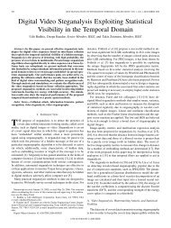
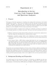
We first <strong>in</strong>vestigate the NMSE, def<strong>in</strong>ed <strong>in</strong> (29) between the true and estimated channels. The NMSE as<br />
a function of SNR is shown <strong>in</strong> Figure 1 <strong>for</strong> w<strong>in</strong>dow sizes 50, 100, 300 and 500. As expected, the NMSE<br />
is a decreas<strong>in</strong>g function of SNR. Although it is true that, <strong>in</strong> theory, cumulant estimates <strong>for</strong> white Gaussian
12<br />
NMSE vs. SNR us<strong>in</strong>g n−po<strong>in</strong>t cumulant estimates <strong>in</strong> a time−<strong>in</strong>variant channel<br />
50−po<strong>in</strong>t Cumulant Estimates<br />
100−po<strong>in</strong>t Cumulant Estimates<br />
300−po<strong>in</strong>t Cumulant Estimates<br />
500−po<strong>in</strong>t Cumulant Estimates<br />
10 −1<br />
10 −2<br />
SNR<br />
NMSE<br />
2 4 6 8 10 12 14 16 18 20<br />
Fig. 1.<br />
Time Invariant <strong>Channel</strong>. NMSE vs. SNR us<strong>in</strong>g 50, 100, 300 and 500 po<strong>in</strong>t cumulant estimates.<br />
noise are zero and the channel estimates should be <strong>in</strong>sensitive to SNR, this occurs when the number of<br />
po<strong>in</strong>ts used <strong>in</strong> the cumulant estimates is very large (we note here that 4 th order cumulants require a very<br />
large number of samples, of the order of thousands or more, <strong>for</strong> the estimated cumulants to converge to<br />
their true statistics. However, we do not require such a large number of samples to get fairly accurate<br />
channel estimates). When us<strong>in</strong>g a realistic number of samples, however, noise affects the accuracy of the<br />
estimation, and the channel estimates are sensitive to SNR. Figure 1 also <strong>in</strong>dicates that, as expected, the<br />
NMSE is a function of w<strong>in</strong>dow size: <strong>in</strong> a static environment, <strong>in</strong>creas<strong>in</strong>g the w<strong>in</strong>dow size will improve<br />
the per<strong>for</strong>mance of the algorithm.<br />
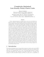
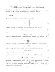
The proposition <strong>in</strong> Section IV-C is verified <strong>in</strong> Figure 2. The figure plots the NMSE of the channel<br />
estimate as a function of B, the number of samples used to estimate the cumulant matrix. The channel<br />
estimates <strong>in</strong> this plot were obta<strong>in</strong>ed from only one cumulant matrix; the NMSE per<strong>for</strong>mance is thus<br />
expectedly slightly worse than that obta<strong>in</strong>ed <strong>in</strong> Figure 1, where the channel estimate was obta<strong>in</strong>ed by<br />
averag<strong>in</strong>g over 2K estimates from 2K cumulant matrices. Because the expression is only valid <strong>for</strong> dist<strong>in</strong>ct<br />
eigenvalues (which are identical <strong>for</strong> equivalent channel magnitudes), it is not accurate when the channel<br />
magnitudes become very close. For this reason, the difference between the channel magnitudes is restricted<br />
to 0.2 and above. The analytical expression approaches the simulated curve as B <strong>in</strong>creases. This is as
13<br />
Actual and Predicted NMSE vs. N<br />
10 −1 N − Number of Po<strong>in</strong>ts <strong>in</strong> the Cumulant Estimate<br />
Actual NMSE<br />
Predicted NMSE<br />
Normalized Mean Squared Error (NMSE)<br />
10 −2<br />
10 −3<br />
0 500 1000 1500 2000 2500 3000<br />
Fig. 2.<br />
Time-Vary<strong>in</strong>g <strong>Channel</strong>. NMSE vs. number of po<strong>in</strong>ts used <strong>in</strong> cumulant estimates.<br />
expected, s<strong>in</strong>ce the approximations used to obta<strong>in</strong> (30) are based on a large B.<br />
<strong>Channel</strong> estimation is one important step towards decod<strong>in</strong>g the transmitted data. From a communication<br />
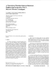
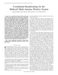
po<strong>in</strong>t of view, it is the BER that is f<strong>in</strong>ally important. The next plot, shown <strong>in</strong> Fig. 3 demonstrates the<br />
efficacy of the channel estimation <strong>in</strong> terms of the result<strong>in</strong>g BER. The BER is compared to that obta<strong>in</strong>ed<br />
by the clairvoyant receiver, which has knowledge of the true channel. As with the NMSE plots, the results<br />
are shown <strong>for</strong> w<strong>in</strong>dow sizes 50, 100, 300 and 500.<br />
Depend<strong>in</strong>g on the number of po<strong>in</strong>ts used <strong>in</strong> cumulant estimates, the system BER, when us<strong>in</strong>g estimated<br />
channels, closely tracks that of the clairvoyant receiver. With 300 and 500-po<strong>in</strong>t cumulant estimates result<br />
<strong>in</strong> almost equivalent BER curves less than 1 dB from the Clairvoyant BER curve. As expected, <strong>in</strong> block<br />
fad<strong>in</strong>g channels, the per<strong>for</strong>mance of the algorithm can always be improved by <strong>in</strong>creas<strong>in</strong>g the number of<br />
po<strong>in</strong>ts used <strong>in</strong> cumulant estimates.<br />
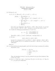
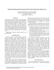
In Figure 4, we compare our scheme to that presented <strong>in</strong> [14] <strong>in</strong> terms of BER. To obta<strong>in</strong> results <strong>for</strong><br />
this algorithm, we use a precod<strong>in</strong>g matrix <strong>for</strong> BPSK symbols D = diag( √ 0.4, √ 1.6, 0, 0. In [14], this<br />
matrix, used <strong>for</strong> QPSK symbols, is chosen <strong>in</strong> an ad hoc fashion; we thus did not optimize this matrix,<br />
but chose a similar one.<br />
The figure demonstrates that our algorithm outper<strong>for</strong>ms the scheme based on covariance estimates by<br />
2 dB. The improved per<strong>for</strong>mance of our cumulant scheme is due to the decreased sensitivity to noise
14<br />
BER vs. SNR us<strong>in</strong>g n−po<strong>in</strong>t cumulant estimates <strong>in</strong> a time−<strong>in</strong>variant channel<br />
50−po<strong>in</strong>t Cumulant Estimates<br />
100−po<strong>in</strong>t Cumulant Estimates<br />
300−po<strong>in</strong>t Cumulant Estimates<br />
500−po<strong>in</strong>t Cumulant Estimates<br />
Clairvoyant Receiver<br />
10 −1 SNR<br />
10 −2<br />
BER<br />
10 −3<br />
10 −4<br />
2 4 6 8 10 12 14 16 18 20<br />
Fig. 3.<br />
Time Invariant <strong>Channel</strong>. BER vs. SNR us<strong>in</strong>g 50, 100, 300 and 500 po<strong>in</strong>t cumulant estimates.<br />
BER vs. SNR us<strong>in</strong>g n−po<strong>in</strong>t cumulant and covariance estimates <strong>in</strong> a time−<strong>in</strong>variant channel<br />
10 −1 SNR<br />
100−po<strong>in</strong>t Covariance Estimates<br />
100−po<strong>in</strong>t Cumulant Estimates<br />
300−po<strong>in</strong>t Covariance Estimates<br />
300−po<strong>in</strong>t Cumulant Estimates<br />
Clairvoyant Receiver<br />
10 −2<br />
BER<br />
10 −3<br />
10 −4<br />
2 4 6 8 10 12 14 16 18 20<br />
Fig. 4.<br />
Time Invariant <strong>Channel</strong>. BER vs. SNR us<strong>in</strong>g 100 and 300 po<strong>in</strong>t cumulant estimates.
15<br />
NMSE vs. SNR us<strong>in</strong>g n−po<strong>in</strong>t cumulant and covariance estimates <strong>in</strong> a time−<strong>in</strong>variant channel<br />
10 0 SNR<br />
100−po<strong>in</strong>t Covariance Estimates<br />
100−po<strong>in</strong>t Cumulant Estimates<br />
300−po<strong>in</strong>t Covariance Estimates<br />
300−po<strong>in</strong>t Cumulant Estimates<br />
10 −1<br />
NMSE<br />
10 −2<br />
10 −3<br />
0 2 4 6 8 10 12 14 16 18 20<br />
Fig. 5.<br />
Time Invariant <strong>Channel</strong>. BER vs. SNR us<strong>in</strong>g 100 and 300 po<strong>in</strong>t cumulant estimates.<br />
of higher order cumulants, and the elim<strong>in</strong>ation of the requirement <strong>for</strong> data precod<strong>in</strong>g. This improved<br />
per<strong>for</strong>mance is obta<strong>in</strong>ed, of course, at the price of <strong>in</strong>creased complexity.<br />
B. Time-Vary<strong>in</strong>g <strong>Channel</strong><br />
The efficacy of the proposed channel estimation algorithm is now exam<strong>in</strong>ed when used <strong>in</strong> a time-vary<strong>in</strong>g<br />
fad<strong>in</strong>g environment. The example is based on two transmit antennas and the Alamouti <strong>STBC</strong>. The data is<br />
sampled at a rate of 20 MHz and is modulated us<strong>in</strong>g a carrier with a frequency of 5.5 GHz. The mobile is<br />
assumed to be mov<strong>in</strong>g at 100 km/h. Clearly, such channels are of practical importance and better reflect<br />
the real world than the block fad<strong>in</strong>g model used <strong>in</strong> Section V-A.<br />
For each Monte Carlo run, 2×10 6 bits are corrupted by the time vary<strong>in</strong>g channel. The channel estimate<br />
<strong>for</strong> a particular w<strong>in</strong>dow of data is obta<strong>in</strong>ed from the cumulant estimate result<strong>in</strong>g from that same w<strong>in</strong>dow.<br />
<strong>Channel</strong> estimates <strong>in</strong> one w<strong>in</strong>dow are fixed, but change from w<strong>in</strong>dow to w<strong>in</strong>dow. To correctly identify<br />
the channels, a pilot symbol is <strong>in</strong>serted at the beg<strong>in</strong>n<strong>in</strong>g of every w<strong>in</strong>dow. We focus here on the BER,<br />
which is more mean<strong>in</strong>gful <strong>in</strong> terms of practical implications. The results are averaged over 250 Monte<br />
Carlo runs.<br />
The BER <strong>for</strong> w<strong>in</strong>dow sizes of 50, 100, 300 and 500 are shown <strong>in</strong> Fig. 6. Unlike <strong>in</strong> the block fad<strong>in</strong>g<br />
example, the estimates obta<strong>in</strong>ed us<strong>in</strong>g 300-po<strong>in</strong>t w<strong>in</strong>dows outper<strong>for</strong>m those obta<strong>in</strong>ed us<strong>in</strong>g 500-po<strong>in</strong>t
16<br />
BER vs. SNR us<strong>in</strong>g n−po<strong>in</strong>t cumulant estimates <strong>in</strong> a time−vary<strong>in</strong>g channel<br />
50−po<strong>in</strong>t Cumulant Estimates<br />
100−po<strong>in</strong>t Cumulant Estimates<br />
300−po<strong>in</strong>t Cumulant Estimates<br />
500−po<strong>in</strong>t Cumulant Estimates<br />
Clairvoyant Receiver<br />
10 −1 SNR<br />
10 −2<br />
BER<br />
10 −3<br />
10 −4<br />
2 4 6 8 10 12 14 16 18 20<br />
Fig. 6.<br />
Time-Vary<strong>in</strong>g <strong>Channel</strong>. BER vs. SNR us<strong>in</strong>g 50, 100, 300 and 500 po<strong>in</strong>t cumulant estimates.<br />
w<strong>in</strong>dows at higher SNR. This occurs because when the channel changes over time, the cumulant estimate<br />
does not necessarily become more accurate <strong>for</strong> longer <strong>in</strong>puts. The variation <strong>in</strong> signal statistics there<strong>for</strong>e<br />
imposes a limit on the maximum number of po<strong>in</strong>ts that can be used <strong>in</strong> cumulant estimates. The faster<br />
these channel variations, the fewer the po<strong>in</strong>ts that can be used.<br />
In Figure 7, we compare BER per<strong>for</strong>mance of our scheme to that that of [14] <strong>in</strong> time-vary<strong>in</strong>g channels.<br />
This comparison is important, s<strong>in</strong>ce covariance estimates are assumed to require less data than cumulant<br />
estimates; it is thus conceivable that the comparison could change <strong>in</strong> time-vary<strong>in</strong>g channels. The figure<br />
demonstrates, however, that the number of po<strong>in</strong>ts required to estimate cumulants and then to obta<strong>in</strong> accurate<br />
channel estimates, are sufficiently low to not be affected by the vary<strong>in</strong>g channel. The BER superiority of<br />
our proposed scheme over the scheme <strong>in</strong> [14] holds <strong>in</strong> this scenario.<br />
VI. CONCLUSIONS<br />
This paper presents a bl<strong>in</strong>d channel estimation algorithm <strong>for</strong> orthogonal space-time block coded data<br />
<strong>in</strong> the important <strong>MISO</strong> situation, i.e., <strong>in</strong> systems us<strong>in</strong>g only a s<strong>in</strong>gle receive antenna. It is shown that the<br />
algorithm outper<strong>for</strong>ms <strong>in</strong> terms of BER the only other exist<strong>in</strong>g algorithm applicable to this scenario. A<br />
significant cost of the algorithm is the complexity <strong>in</strong>volved <strong>in</strong> estimat<strong>in</strong>g the required cumulants. Cumulant<br />
estimates are generally assumed to be impractical s<strong>in</strong>ce they require too many samples to be effective. Very
17<br />
BER vs. SNR us<strong>in</strong>g n−po<strong>in</strong>t cumulant and covariance estimates <strong>in</strong> a time−vary<strong>in</strong>g channel<br />
100−po<strong>in</strong>t Covariance Estimates<br />
100−po<strong>in</strong>t Cumulant Estimates<br />
300−po<strong>in</strong>t Covariance Estimates<br />
300−po<strong>in</strong>t Cumulant Estimates<br />
Clairvoyant Receiver<br />
10 −1 SNR<br />
10 −2<br />
BER<br />
10 −3<br />
10 −4<br />
2 4 6 8 10 12 14 16 18 20<br />
Fig. 7.<br />
Time-Vary<strong>in</strong>g <strong>Channel</strong>. BER vs. SNR us<strong>in</strong>g 50, 100, 300 and 500 po<strong>in</strong>t cumulant estimates.<br />
good estimation results, however, are obta<strong>in</strong>ed when us<strong>in</strong>g as few as 100 − 300 po<strong>in</strong>ts <strong>in</strong> the cumulant<br />
estimates. The numerical simulations prove that even if us<strong>in</strong>g the the sample number of samples, the<br />
cumulant-based scheme presented here outper<strong>for</strong>ms the previously proposed scheme based on covariance<br />
estimates.<br />
APPENDIX I<br />
CHANNEL MAGNITUDES<br />
The channel magnitudes can be obta<strong>in</strong>ed from the non-zero eigenvalues λ j as follows:<br />
λ j = γ 4 ||h|| 2 Ff j , (31)<br />
= γ 4 |h kj | 2 ||h|| 2 F,<br />
where f j represents the the j th non-zero diagonal entry of matrix F k def<strong>in</strong>ed <strong>in</strong> (20) and (21) <strong>for</strong> complex<br />
and real data, respectively. ||h|| 2 F is found by summ<strong>in</strong>g the non-zero eigenvalues λ j of each cumulant
18<br />
matrix, C [k]<br />
4 :<br />
2K∑<br />
k=1 j=1<br />
L∑<br />
λ j =<br />
2K∑<br />
k=1 j=1<br />
L∑<br />
(γ 4 |h kj | 2 ||h|| 2 F) = αγ 4 ||h|| 4 F. (32)<br />
⇒ ||h|| 2 F =<br />
1<br />
√<br />
1<br />
γ ∑ . (33)<br />
L<br />
α 4 j=1 λ j<br />
Here, α is a parameter dependent on the constellation: α = 2 <strong>for</strong> real and α = 4 <strong>for</strong> complex constellations.<br />
APPENDIX II<br />
NMSE ANALYSIS<br />
In this appendix we show that <strong>for</strong> the Alamouti <strong>STBC</strong> with one receive antenna and <strong>for</strong> a particular<br />
channel pair, the NMSE can be approximated by (30). We assume here a high SNR region, and thus<br />
channel estimation errors are due only to estimation errors due to a f<strong>in</strong>ite number of samples, and are<br />
<strong>in</strong>sensitive to noise. In this section, we do not separate the real and imag<strong>in</strong>ary parts of the received signal,<br />
and use the model<br />
⎡ ⎤ ⎡ ⎤<br />
r = ⎣ r 1<br />
⎦ = ⎣ h 1s 1 + h 2 s 2<br />
⎦ + w, (34)<br />
r 2 −h 1 s ∗ 2 + h 2 s ∗ 1<br />
⎡ ⎤ ⎡ ⎤<br />
⇒ r ′ = ⎣ r 1<br />
⎦ = H c<br />
⎣ s 1<br />
⎦ + w, (35)<br />
s 2<br />
r ∗ 2<br />
where<br />
H c =<br />
⎡<br />
⎣ h 1 h 2<br />
h ∗ 2 −h ∗ 1<br />
⎤<br />
⎦. (36)<br />
Without loss of generality, we def<strong>in</strong>e v 1 and v 2 as the normalized eigenvectors of the cumulant matrix<br />
C 4 , such that v H 1 v 1 = v H 2 v 2 = 1. v 1 and v 2 correspond to the scaled columns of the channel matrix H c ,<br />
such that<br />
v 1 =<br />
⎡<br />
1<br />
√ ⎣ h 0<br />
|h0 | 2 + |h 1 | 2<br />
h ∗ 1<br />
⎤<br />
⎦, v 1 =<br />
⎡<br />
1<br />
√ ⎣ h 1<br />
|h0 | 2 + |h 1 | 2<br />
−h ∗ 0<br />
⎤<br />
⎦. (37)
19<br />
Def<strong>in</strong><strong>in</strong>g ˆv 1 and ˆv 2 as the eigenvectors of the estimated cumulant matrix, Ĉ4, and δ vj = ˆv j −v j as the<br />
error between them, the NMSE of the estimated channels is exactly δ H v 1<br />
δ v1 = δ H v 2<br />
δ v2 . Because the two are<br />
equivalent, we will focus on the error <strong>in</strong> the first eigenvector, δ H v 1<br />
δ v1 .<br />
In [19], Yuen and Friedlander derive the covariance matrix of the error between the estimated and true<br />
eigenvectors of a cumulant matrix. The expression is valid <strong>in</strong> cases where the cumulant matrix has dist<strong>in</strong>ct<br />
values. Applied to the problem <strong>in</strong> this work, the expression becomes<br />
δ H v 1<br />
δ v1 =<br />
1<br />
2∑<br />
(α 1 − α 2 ) 2<br />
2∑<br />
2∑<br />
a 1 =1 a 2 =1 b 1 =1 b 2 =1<br />
2∑<br />
v2,a ∗ 1<br />
v 1,a2 v 2,b1 v1,b ∗ 2<br />
E{(C 4 − Ĉ 4 ) a1 a 2<br />
(C 4 − Ĉ 4 ) b1 b 2<br />
, (38)<br />
where the quantity v i,j is def<strong>in</strong>ed as the j th element of vector i, and (C 4 − Ĉ 4 ) ij is the ij th element of<br />
(C 4 − Ĉ 4 ). C 4 is as def<strong>in</strong>ed <strong>in</strong> (17).<br />
In [20], Porat and Friedlander derive expressions <strong>for</strong> the covariance matrix of fourth-order sample<br />
cumulants of zero-mean and symmetrically distributed signals. The analysis <strong>in</strong> [20] assumes that a large<br />
number of data po<strong>in</strong>ts, B, are used <strong>in</strong> the estimation of the cumulant matrix. In this analysis, the <strong>in</strong>put<br />
to the <strong>for</strong>th-order cumulants is the received signal <strong>in</strong> (II). This signal r is both zero-mean and symmetric<br />
<strong>for</strong> both BPSK and QAM <strong>in</strong>put signals s, and thus the expression derived <strong>in</strong> [20] is valid. It is repeated<br />
here <strong>for</strong> convenience.<br />
B × E {[c 4 (k 1 ,k 2 ,l ∗ 1,l ∗ 2) − ĉ 4 (k 1 ,k 2 ,l ∗ 1,l ∗ 2)] · [c 4 (m 1 ,m 2 ,n ∗ 1,n ∗ 2) − ĉ 4 (m 1 ,m 2 ,n ∗ 1,n ∗ 2)]}<br />
≈ µ 8 (k 1 ,k 2 ,m 1 ,m 2 ,l ∗ 1,l ∗ 2,n ∗ 2,n ∗ 2)<br />
− ∑ 2<br />
p=1<br />
∑ 2<br />
q=1 µ 2(m 3−p ,n ∗ 3−q) µ 6 (k 1 ,k 2 ,m p ,l ∗ 1,l ∗ 2,n ∗ q)<br />
− ∑ 2<br />
i=1<br />
∑ 2<br />
j=1 µ 2(k ∗ 3−i,l ∗ 3−j) µ 6 (m 1 ,m 2 ,k i ,n ∗ 1,n ∗ 2,l ∗ j)<br />
+ ∑ 2<br />
i=1<br />
∑ 2<br />
j=1<br />
∑ 2<br />
p=1<br />
∑ 2<br />
q=1 µ 2(m 3−p ,n ∗ 3−q) µ 2 (k 3−i ,l ∗ 3−j) µ 4 (k i ,m p ,l ∗ j,n ∗ q)<br />
− [[u 4 (k 1 ,k 2 ,l ∗ 1,l ∗ 2) − 2u 2 (k 1 ,l ∗ 1)u 2 (k 2 ,l ∗ 2) − 2u 2 (k 1 ,l ∗ 2)u 2 (k 2 ,l ∗ 1)]<br />
(39)<br />
· [u 4 (m 1 ,m 2 ,n ∗ 1,n ∗ 2) − 2u 2 (m 1 ,n ∗ 1)u 2 (m 2 ,n ∗ 2) − 2u 2 (m 1 ,n ∗ 2)u 2 (m 2 ,n ∗ 1)]].<br />
To determ<strong>in</strong>e the expression <strong>in</strong> (38), the 16 correspond<strong>in</strong>g cumulant covariances must be determ<strong>in</strong>ed<br />
us<strong>in</strong>g (39). This can be simplified us<strong>in</strong>g the fact that (C 4 − Ĉ 4 ) is Hermitian, and thus, <strong>for</strong> example<br />
(C 4 − Ĉ 4 ) 11 (C 4 − Ĉ 4 ) ∗ 12 = (C 4 − Ĉ 4 ) 21 (C 4 − Ĉ 4 ) ∗ 11. (40)<br />
The calculations <strong>for</strong> the necessary cumulant covariances are tedious but straight<strong>for</strong>ward, and the results
20<br />
are given below:<br />
E{(C 4 − Ĉ 4 ) 11 (C 4 − Ĉ 4 ) 11 } =γ 2 4(h 4 0h ∗4<br />
1 + h ∗4<br />
0 h 4 1 + 18|h 0 | 4 |h 1 | 4 + 8|h 0 | 2 |h 1 | 6 + 8|h 0 | 6 |h 1 | 2 ) (41)<br />
E{(C 4 − Ĉ 4 ) 22 (C 4 − Ĉ 4 ) 22 } =γ 2 4(h 4 0h ∗4<br />
1 + h ∗4<br />
0 h 4 1 + 2|h 0 | 4 |h 1 | 4 ) (42)<br />
E{(C 4 − Ĉ 4 ) 11 (C 4 − Ĉ 4 ) 12 } =γ 2 4(−h 5 0h ∗3<br />
1 + h ∗3<br />
0 h 5 1 − 3h 0 h 1 |h 0 | 4 |h 1 | 2<br />
+ 3h 0 h 1 |h 0 | 2 |h 1 | 4 + 2h 0 h 1 |h 1 | 6 − 2h 0 h 1 |h 1 | 6 ) (43)<br />
E{(C 4 − Ĉ 4 ) 12 (C 4 − Ĉ 4 ) ∗ 12} =γ 2 4(−h 4 0h ∗4<br />
1 − h ∗4<br />
0 h 4 1 + 3|h 0 | 6 |h 1 | 2 + 3|h 0 | 2 |h 1 | 6 + 2|h 0 | 4 |h 1 | 4 ) (44)<br />
E{(C 4 − Ĉ 4 ) 11 (C 4 − Ĉ 4 ) 22 } =γ 2 4(−h 4 0h ∗4<br />
1 − h ∗4<br />
0 h 4 1 − 2|h 0 | 4 |h 1 | 4 ) (45)<br />
E{(C 4 − Ĉ 4 ) 12 (C 4 − Ĉ 4 ) 12 } =γ 2 4(−6h 2 0h 2 1|h 0 | 2 |h 1 | 2 − 2h 2 0h 2 1(|h 0 | 4 + |h 1 | 4 ) + h 6 0h ∗2<br />
1 + h ∗2<br />
0 h 6 1) (46)<br />
E{(C 4 − Ĉ 4 ) 22 (C 4 − Ĉ 4 ) 12 } =γ 2 4(h 5 0h ∗3<br />
1 − h ∗3<br />
0 h 5 1 − h 0 h 1 |h 0 | 2 |h 1 | 4 + h 0 h 1 |h 0 | 4 |h 1 | 2 ) (47)<br />
Us<strong>in</strong>g (41) - (47), the expression <strong>for</strong> the eigenvalues of the cumulant matrix given <strong>in</strong> (32) and us<strong>in</strong>g (37)<br />
are substituted <strong>in</strong> (38), results <strong>in</strong><br />
NMSE ≈ |h 0| 4 + 3|h 0 | 2 |h 1 | 2 + |h 1 | 4<br />
B(|h 0 | 2 − |h 1 |) 2 ) 2 (48)<br />
REFERENCES<br />
[1] V. Tarokh, N. Seshadri, and A. R. Calderbank, “Spacetime codes <strong>for</strong> high data rate wireless communication: Per<strong>for</strong>mance criterion and<br />
code construction,” IEEE Transactions on In<strong>for</strong>mation Theory, vol. 44, pp. 744–765, March 1998.<br />
[2] V. Tarokh, H. Jafarkhani, and A. R. Calderbank, “Spacetime block codes from orthogonal designs,” IEEE Transactions on In<strong>for</strong>mation<br />
Theory, vol. 45, pp. 1456–1467, July 1999.<br />
[3] S. M. Alamouti, “A simple transmit diversity technique <strong>for</strong> wireless communications,” IEEE Journal on Select Areas <strong>in</strong> Communications,<br />
vol. 16, pp. 1451–1458, August 1998.<br />
[4] Z. D<strong>in</strong>g and Y. Li, <strong>Bl<strong>in</strong>d</strong> Equalization and Identification. Marcel Dekker, 2001.<br />
[5] C. Budianu and L. Tong, “<strong>Channel</strong> estimation <strong>for</strong> space-time orthogonal block code,” <strong>in</strong> Proc. of International Conference on<br />
Communications, pp. 1127–1131, June 2001.<br />
[6] E. G. Larsson, P. Stoica, and J. Li, “<strong>Orthogonal</strong> space-time block codes: maximum likelihood detection <strong>for</strong> unknown channels and<br />
unstructured <strong>in</strong>terferences,” IEEE Transactions on Signal Process<strong>in</strong>g, vol. 51, pp. 362–372, Feb 2003.<br />
[7] N. Ammar and Z. D<strong>in</strong>g, “<strong>Channel</strong> estimation under space-time block-code transmission,” <strong>in</strong> Proc. of Sensor Array and Multichannel<br />
Signal Process<strong>in</strong>g Workshop, pp. 422–426, August 2002.<br />
[8] A. L. Sw<strong>in</strong>dlehurst and G. Leus, “<strong>Bl<strong>in</strong>d</strong> and semi-bl<strong>in</strong>d equalization <strong>for</strong> generalized space-time block codes,” IEEE Transactions on<br />
Signal Process<strong>in</strong>g, vol. 50, pp. 2489–2498, October 2002.<br />
[9] P. Stoica and G. Ganesan, “Space-time block-codes: tra<strong>in</strong>ed, bl<strong>in</strong>d and semi-bl<strong>in</strong>d detection,” <strong>in</strong> Proc. of International Conference on<br />
Acoustics, Speech and Signal Process<strong>in</strong>g, pp. 1609–1612, 2002.
21<br />
[10] E. G. Larsson, P. Stoica, and J. Li, “On maximum-likelihood detection and decod<strong>in</strong>g <strong>for</strong> space-time cod<strong>in</strong>g systems,” IEEE Transactions<br />
on Signal Process<strong>in</strong>g, vol. 50, pp. 937 – 944, April 2002.<br />
[11] W.-K. Ma, P. C. Ch<strong>in</strong>g, T. N. Davidson, and X. G. Xia, “<strong>Bl<strong>in</strong>d</strong> maximum-likelihood decod<strong>in</strong>g <strong>for</strong> orthogonal space-time block codes:<br />
a semidef<strong>in</strong>ite relaxation approach,” <strong>in</strong> Proc. of the IEEE Global Telecommunications Conference, p. 2094 2098, Dec 2003.<br />
[12] W.-K. Ma, B.-N. Vo, and T. N. Davidson, “On implement<strong>in</strong>g the bl<strong>in</strong>d ML receiver <strong>for</strong> orthogonal space-time block codes,” <strong>in</strong> Proc.<br />
of the IEEE International Conference on Acoustics, Speech, and Signal Process<strong>in</strong>g, March 2005.<br />
[13] W.-K. Ma, V. B.-N. Vo, T. N. Davidson, and P.-C. Ch<strong>in</strong>g, “<strong>Bl<strong>in</strong>d</strong> ML detection of orthogonal space-time block codes: efficient highper<strong>for</strong>mance<br />
implementations,” IEEE Transactions on Signal Process<strong>in</strong>g, vol. 54, pp. 738 – 751, Feb 2006.<br />
[14] S. Shahbazpanahi, A. B. Gershman, and J. H. Manton, “Closed-<strong>for</strong>m bl<strong>in</strong>d MIMO channel estimation <strong>for</strong> orthogonal space-time block<br />
codes,” IEEE Transactions on signal process<strong>in</strong>g, vol. 53, pp. 4506 – 4517, December 2005.<br />
[15] Z. D<strong>in</strong>g and J. Liang, “A cumulant matrix subspace algorithm <strong>for</strong> bl<strong>in</strong>d s<strong>in</strong>gle FIR channel identification,” IEEE Transactions on Signal<br />
Process<strong>in</strong>g, vol. 49, pp. 325–333, February 2001.<br />
[16] C. L. Nikias and A. P. Petropulu, Higher-Order Spectral Analysis. PTR Prentice Hall, 1993.<br />
[17] S. Shahbazpanahi, A. B. Gershman, and J. H. Manton, “A l<strong>in</strong>ear precod<strong>in</strong>g approach to resolve ambiguity of bl<strong>in</strong>d decod<strong>in</strong>g of orthogonal<br />
space-time block codes <strong>in</strong> slowly fad<strong>in</strong>g channels,” <strong>in</strong> IEEE Workshop on Signal Process<strong>in</strong>g Advances <strong>in</strong> Wireless Communications,<br />
SPAWC 2004, pp. 228 – 232, July 2004.<br />
[18] G. W. C. Leung and D. Hatz<strong>in</strong>akos, “Implementation aspects of various higher-order statistics estimators,” J. Frankl<strong>in</strong> Institute,<br />
vol. 333(B), no. 3, pp. 349–367, 1996.<br />
[19] N. Yuen and B. Friedlander, “Asymptotic per<strong>for</strong>mance analysis of esprit, higher order esprit, and virtual esprit algorithms,” IEEE<br />
Transactions on Signal Process<strong>in</strong>g, vol. 44, pp. 2537 – 2550, October 1996.<br />
[20] B. Porat and B. Friedlander, “Direction f<strong>in</strong>d<strong>in</strong>g algorithms based on high-order statistics,” IEEE Transactions on Signal Process<strong>in</strong>g,<br />
vol. 39, pp. 2016 – 2024, September 1991.