Greville's Method for Preconditioning Least Squares ... - Projects

4
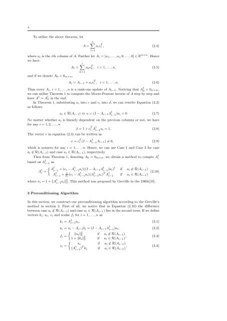
To utilize the above theorem, let
A =
n∑
a i e T i , (2.4)
i=1
where a i is the ith column of A. Further let A i = [a 1 , . . . , a i , 0, . . . , 0] ∈ R m×n . Hence
we have
i∑
A i = a k e T k , i = 1, . . . , n, (2.5)
and if we denote A 0 = 0 m×n ,
k=1
A i = A i−1 + a i e T i , i = 1, . . . , n. (2.6)
Thus every A i , i = 1, . . . , n is a rank-one update of A i−1 . Noticing that A † 0 = 0 n×m,
we can utilize Theorem 1 to compute the Moore-Penrose inverse of A step by step and
have A † = A † n in the end.
In Theorem 1, substituting a i into c and e i into d, we can rewrite Equation (2.2)
as follows.
a i ∈ R(A i−1 ) ⇔ u = (I − A i−1 A † i−1 )a i = 0 (2.7)
No matter whether a i is linearly dependent on the previous columns or not, we have
for any i = 1, 2, . . . , n
β = 1 + e T i A † i−1 a i = 1. (2.8)
The vector v in equation (2.3) can be written as
v = e T i (I − A † i−1 A i−1) ≠ 0, (2.9)
which is nonzero for any i = 1, . . . , n. Hence, we can use Case 1 and Case 3 for case
a i ∉ R(A i−1 ) and case a i ∈ R(A i−1 ), respectively.
Then from Theorem 1, denoting A 0 = 0 m×n , we obtain a method to compte A † i
based on A † i−1 as
A † i = { A
†
i−1 + (e i − A † i−1 a i)((I − A i−1 A † i−1 )a i) † if a i ∉ R(A i−1 )
A † i−1 + 1 σ i
(e i − A † i−1 a i)(A † i−1 a i) T A † i−1 if a i ∈ R(A i−1 ) (2.10)
where σ i = 1 + ‖A † i−1 a i‖ 2 2. This method was proposed by Greville in the 1960s[13].
3 Preconditioning Algorithm
In this section, we construct our preconditioning algorithm according to the Greville’s
method in section 2. First of all, we notice that in Equation (2.10) the difference
between case a i ∉ R(A i−1 ) and case a i ∈ R(A i−1 ) lies in the second term. If we define
vectors k i , u i , v i and scalar f i for i = 1, . . . , n as
k i = A † i−1 a i, (3.1)
u i = a i − A i−1 k i = (I − A i−1 A † i−1 )a i, (3.2)
{ ‖ui ‖ 2 2 if a
f i =
i ∉ R(A i−1 )
1 + ‖k i ‖ 2 2 if a i ∈ R(A i−1 ) , (3.3)
{
u i if a i ∉ R(A i−1 )
v i =
(A † i−1 )T k i if a i ∈ R(A i−1 ) , (3.4)