Greville's Method for Preconditioning Least Squares ... - Projects
Greville's Method for Preconditioning Least Squares ... - Projects
Greville's Method for Preconditioning Least Squares ... - Projects
Create successful ePaper yourself
Turn your PDF publications into a flip-book with our unique Google optimized e-Paper software.
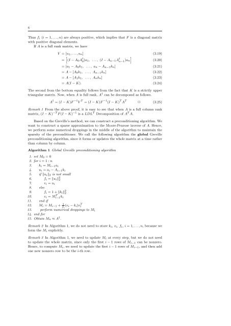
6<br />
Thus f i (i = 1, . . . , n) are always positive, which implies that F is a diagonal matrix<br />
with positive diagonal elements.<br />
If A is a full rank matrix, we have<br />
V = [u 1 , . . . , u n] (3.19)<br />
]<br />
=<br />
[(I − A 0 A † 0 )a 1, . . . , (I − A n−1 A † n−1 )an (3.20)<br />
= [a 1 − A 0 k 1 , . . . , a n − A n−1 k n] (3.21)<br />
= A − [A 0 k 1 , . . . , A n−1 k n] (3.22)<br />
= A − [A 1 k 1 , . . . , A nk n] (3.23)<br />
= A(I − K). (3.24)<br />
The second from the bottom equality follows from the fact that K is a strictly upper<br />
triangular matrix. Now, when A is full rank, A † can be decomposed as follows.<br />
A † = (I − K)F −1 V T = (I − K)F −1 (I − K) T A T ✷ (3.25)<br />
Remark 1 From the above proof, it is easy to see that when A is a full column rank<br />
matrix, (I − K) −T F (I − K) −1 is a LDL T Decomposition of A T A.<br />
Based on the Greville’s method, we can construct a preconditioning algorithm. We<br />
want to construct a sparse approximation to the Moore-Penrose inverse of A. Hence,<br />
we per<strong>for</strong>m some numerical droppings in the middle of the algorithm to maintain the<br />
sparsity of the preconditioner. We call the following algorithm the global Greville<br />
preconditioning algorithm, since it <strong>for</strong>ms or updates the whole matrix at a time rather<br />
than column by column.<br />
Algorithm 1 Global Greville preconditioning algorithm<br />
1. set M 0 = 0<br />
2. <strong>for</strong> i = 1 : n<br />
3. k i = M i−1 a i<br />
4. u i = a i − A i−1 k i<br />
5. if ‖u i ‖ 2 is not small<br />
6. f i = ‖u i ‖ 2 2<br />
7. v i = u i<br />
8. else<br />
9. f i = 1 + ‖k i ‖ 2 2<br />
10. v i = Mi−1 T k i<br />
11. end if<br />
12. M i = M i−1 + f 1 i<br />
(e i − k i )vi<br />
T<br />
13. per<strong>for</strong>m numerical droppings to M i<br />
14. end <strong>for</strong><br />
15. Obtain M n ≈ A † .<br />
Remark 2 In Algorithm 1, we do not need to store k i , v i , f i , i = 1, . . . , n, because we<br />
<strong>for</strong>m the M i explicitly.<br />
Remark 3 In Algorithm 1, we need to update M i at every step, but we do not need<br />
to update the whole matrix, since only the first i − 1 rows of M i−1 can be nonzero.<br />
Hence, to compute M i , we need to update the first i − 1 rows of M i−1 , and then add<br />
one new nonzero row to be the i-th row.


