Robustness Techniques for Feature Extraction - Berlin Chen
Robustness Techniques for Feature Extraction - Berlin Chen
Robustness Techniques for Feature Extraction - Berlin Chen

You also want an ePaper? Increase the reach of your titles
YUMPU automatically turns print PDFs into web optimized ePapers that Google loves.
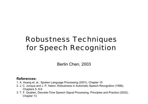
<strong>Robustness</strong> <strong>Techniques</strong><br />
<strong>for</strong> Speech Recognition<br />
<strong>Berlin</strong> <strong>Chen</strong>, 2003<br />
References:<br />
1. X. Huang et. al., Spoken Language Processing (2001), Chapter 10<br />
2. J. C. Junqua and J. P. Haton, <strong>Robustness</strong> in Automatic Speech Recognition (1996),<br />
Chapters 5, 8-9<br />
3. T. F. Quatieri, Discrete-Time Speech Signal Processing, Principles and Practice (2002),<br />
Chapter 13
Introduction<br />
• Classification of Speech Variability in Five Categories<br />
Pronunciation<br />
Variation<br />
Intra-speaker<br />
variability<br />
Linguistic<br />
variability<br />
Inter-speaker<br />
variability<br />
Speaker-independency<br />
Speaker-adaptation<br />
Speaker-dependency<br />
<strong>Robustness</strong><br />
Enhancement<br />
Variability caused<br />
by the environment<br />
Variability caused<br />
by the context<br />
Context-Dependent<br />
Acoustic Modeling<br />
2
Introduction<br />
• The Diagram <strong>for</strong> Speech Recognition<br />
Acoustic Processing Linguistic Processing<br />
Speech<br />
signal<br />
<strong>Feature</strong><br />
<strong>Extraction</strong><br />
Likelihood<br />
computation<br />
Linguistic Network<br />
Decoding<br />
Recognition<br />
results<br />
Acoustic<br />
model model<br />
Language<br />
model model<br />
Lexicon<br />
• Importance of the robustness in speech recognition<br />
– Speech recognition systems must operate in situations with<br />
uncontrollable acoustic environments<br />
– The recognition per<strong>for</strong>mance is often degraded due to the<br />
mismatch in the training and testing conditions<br />
• Varying environmental noises, different speaker characteristics<br />
(sex, age, dialects), different speaking modes (stylistic, Lombard<br />
effect), etc.<br />
3
Introduction<br />
• If a speech recognition system’s accuracy doesn’t degrade<br />
very much under mismatch conditions, the system is called<br />
E<br />
s<br />
E<br />
s 2.5<br />
robust<br />
25dB<br />
= 10 log<br />
10<br />
=> = 10 ≈<br />
– ASR per<strong>for</strong>mance is rather uni<strong>for</strong>m <strong>for</strong> SNRs greater than 25dB, but<br />
there is a very steep degradation as the noise level increases<br />
• Variant noises exist in varying real-world environments<br />
(periordic, impulsive, or wide/narrow band)<br />
• There<strong>for</strong>e, several possible robustness approaches have<br />
been developed to enhance the speech signal, its<br />
spectrum, and the acoustic models as well<br />
– Environment compensation processing (feature-based)<br />
– Environment model adaptation (model-based)<br />
– Inherently robust acoustic features (both model- and feature-based)<br />
• Discriminatively trained acoustic features<br />
E<br />
N<br />
E<br />
N<br />
316<br />
4
The Noise Types<br />
s[m]<br />
h[m]<br />
n[m]<br />
x[m]<br />
A model of the environment.<br />
x<br />
[ m] = s[ m] ∗ h[ m] + n[ m]<br />
X ( ω ) = S( ω ) H ( ω ) + N ( ω )<br />
2<br />
2<br />
2<br />
2<br />
*<br />
X ( ω ) = S( ω ) H ( ω ) + N ( ω ) + 2 Re{ S( ω ) H ( ω ) N ( ω )}<br />
2<br />
2<br />
2<br />
= S( ω ) H ( ω ) + N ( ω ) + 2 S( ω ) H ( ω ) N ( ω ) cos<br />
2<br />
2<br />
2<br />
≈ S( ω ) H ( ω ) + N ( ω )<br />
or P ( ) = P ( ) P ( ) + P ( ) , P()<br />
X<br />
ω<br />
S<br />
ω<br />
H<br />
ω<br />
N<br />
ω ⋅ : power spectrum<br />
or S ( ω ) = S ( ω ) S ( ω ) + S ( ω ) , S ():<br />
power spectrum<br />
⇔<br />
⇔<br />
xx<br />
ss<br />
hh<br />
nn<br />
--<br />
⋅<br />
θ<br />
ω
Additive Noises<br />
• Additive noises can be stationary or non-stationary<br />
– Stationary noises<br />
• Such as computer fan, air conditioning, car noise: the power<br />
spectral density does not change over time (the above noises are<br />
also narrow-band noises)<br />
– Non-stationary noises<br />
• Machine gun, door slams, keyboard clicks, radio/TV, and other<br />
speakers’ voices (babble noise, wide band nose, most difficult): the<br />
statistical properties<br />
change over time<br />
6
Additive Noises<br />
7
Convolutional Noises<br />
• Convolutional noises are mainly resulted from channel<br />
distortion (sometimes called “channel noises”) and are<br />
stationary <strong>for</strong> most cases<br />
– Reverberation, the frequency response of microphone,<br />
transmission lines, etc.<br />
8
Noise Characteristics<br />
• White Noise<br />
– The power spectrum is flat S nn<br />
ω = ,a condition equivalent to<br />
different samples being uncorrelated, R nn<br />
[ m] = qδ<br />
[ m]<br />
– White noise has a zero mean, but can have different distributions<br />
– We are often interested in the white Gaussian noise, as it<br />
resembles better the noise that tends to occur in practice<br />
• Colored Noise<br />
( ) q<br />
– The spectrum is not flat (like the noise captured by a microphone)<br />
– Pink noise<br />
• A particular type of colored nose that has a low-pass nature, as it<br />
has more energy at the low frequencies and rolls off at high<br />
frequency<br />
• E.g., the noise generated by a computer fan, an air conditioner, or<br />
an automobile<br />
9
• Musical Noise<br />
Noise Characteristics<br />
– Musical noise is short sinusoids (tones) randomly distributed<br />
over time and frequency that occur due to the drawback of<br />
original spectral subtraction technique and statistical inaccuracy<br />
in estimating noise magnitude spectrum<br />
• Lombard effect<br />
– A phenomenon by which a speaker increases his vocal effect in<br />
the presence of background noise (the additive noise)<br />
– When a large amount of noise is present, the speaker tends to<br />
shout, which entails not only a high amplitude, but also often<br />
higher pitch, slightly different <strong>for</strong>mants, and a different coloring<br />
(shape) of the spectrum<br />
– The vowel portion of the words will be overemphasized by the<br />
speakers<br />
10
<strong>Robustness</strong> Approaches
Three Basic Categories of Approaches<br />
• Speech Enhancement <strong>Techniques</strong><br />
– Eliminating or reducing the noisy effect on the speech signals,<br />
thus better accuracy with the originally trained models<br />
(Restore the clean speech signals or compensate <strong>for</strong> distortions)<br />
– The feature part is modified while the model part remains<br />
unchanged<br />
• Model-based Noise Compensation <strong>Techniques</strong><br />
– Adjusting (changing) the recognition model parameters (means<br />
and variances) <strong>for</strong> better matching the testing noisy conditions<br />
– The model part is modified while the feature part remains<br />
unchanged<br />
• Inherently Robust Parameters <strong>for</strong> Speech<br />
– Finding robust representation of speech signals less influenced<br />
by additive or channel noise<br />
– Both of the feature and model parts are changed<br />
12
Three Basic Categories of Approaches<br />
• General Assumptions <strong>for</strong> the Noise<br />
– The noise is uncorrelated with the speech signal<br />
– The noise characteristics are fixed during the speech utterance<br />
or vary very slowly (the noise is said to be stationary)<br />
• The estimates of the noise characteristics can be obtained during<br />
non-speech activity<br />
– The noise is supposed to be additive or convolutional<br />
• Per<strong>for</strong>mance Evaluation<br />
– Intelligibility, quality (subjective assessment)<br />
– Distortion between clean and recovered speech (objective<br />
assessment)<br />
– Speech recognition accuracy<br />
13
Spectral Subtraction (SS) S. F. Boll, 1979<br />
• A Speech Enhancement Technique<br />
• Estimate the magnitude (or the power) of clean speech by<br />
explicitly subtracting the noise magnitude (or the power)<br />
spectrum from the noisy magnitude (or power) spectrum<br />
• Basic Assumption of Spectral Subtraction<br />
– The clean speech s [ m]<br />
is corrupted by additive noise n[ m]<br />
– Different frequencies are uncorrelated from each other<br />
– s [ m]<br />
and n[ m]<br />
are statistically independent, so that the power<br />
spectrum of the noisy speech x[ m]<br />
can be expressed as:<br />
P ( ω ) = P ( ω ) + P ( ω )<br />
X<br />
S<br />
N<br />
– To eliminate the additive noise: P ( ω ) = P ( ω ) − P ( ω )<br />
S<br />
X<br />
N<br />
– We can obtain an estimate of P N<br />
( ω ) using the average period of M<br />
frames that known to be just noise:<br />
Pˆ<br />
1<br />
M<br />
M<br />
( ) ∑ − 1<br />
ω = ( ω )<br />
P N N ,i i=<br />
0<br />
14
Spectral Subtraction (SS)<br />
• Problems of Spectral Subtraction<br />
– s [ m]<br />
and n[ m]<br />
are not statistically independent such that the cross<br />
term in power spectrum can not be eliminated<br />
( )<br />
– ω is possibly less than zero<br />
PˆS<br />
– Introduce “musical noise” when<br />
( ω ) ≈ P ( ω )<br />
– Need a robust endpoint (speech/noise/silence) detector<br />
P<br />
X<br />
N<br />
15
Spectral Subtraction (SS)<br />
• Modification: Nonlinear Spectral Subtraction (NSS)<br />
Pˆ<br />
P<br />
S<br />
⎧PX<br />
( ω ) − PN<br />
( ω ),<br />
if PX<br />
( ω ) ≥ PN<br />
( ω )<br />
( ω ) = ⎨<br />
⎩PN<br />
( ω ),<br />
otherwise<br />
( ω ) and P ( ω ): smoothed noisy and noise spectrum<br />
X<br />
N<br />
or<br />
Pˆ<br />
P<br />
φ<br />
⎧P<br />
( ) ( ) ( ) ( ) ( )<br />
X<br />
ω − φ ω , if PX<br />
ω > φ ω + β ⋅ PN<br />
ω<br />
( )<br />
S<br />
ω = ⎨<br />
⎩β<br />
⋅ P ( ω )<br />
N<br />
, otherwise<br />
( ω ) and P ( ω )<br />
X<br />
N<br />
: smoothed noisy and noise<br />
( ω ):<br />
a non - linear function according to SNR<br />
spectrum<br />
16
Spectral Subtraction (SS)<br />
• Spectral Subtraction can be viewed as a filtering<br />
operation<br />
Pˆ<br />
S<br />
( ω ) = P ( ) ( )<br />
X<br />
ω − PN<br />
ω<br />
⎡ P<br />
( )<br />
( )<br />
N<br />
ω<br />
= PX<br />
ω ⎢1<br />
−<br />
P ( ω )<br />
Power Spectrum<br />
P ( )<br />
S<br />
ω<br />
( ω ) + P ( ω )<br />
⎤ ⎡<br />
⎤<br />
⎥ = P ( )<br />
X<br />
ω ⎢<br />
⎥ (supposed that PX<br />
S<br />
+<br />
⎣ X ⎦ ⎣ PS<br />
N ⎦<br />
−1<br />
⎡ 1 ⎤<br />
P<br />
( )<br />
( )<br />
( )<br />
N<br />
ω<br />
= PX<br />
ω ⎢1<br />
+<br />
( R = :instantaneous SNR )<br />
R( )<br />
⎥ ω<br />
⎣ ω ⎦<br />
P ( )<br />
S<br />
ω<br />
∴The time varyingsuppression filter is given approximately by :<br />
( ω) ≈ P ( ω) P ( ω)<br />
N<br />
)<br />
H<br />
( ω)<br />
⎢<br />
⎡ = 1 +<br />
⎣<br />
1<br />
R<br />
( ω)<br />
⎤<br />
⎥<br />
⎦<br />
−1 / 2<br />
Spectrum Domain<br />
17
Wiener Filtering<br />
• A Speech Enhancement Technique<br />
• From the Statistical Point of View<br />
– The process x[ m]<br />
is the sum of the random process s[ m]<br />
and the<br />
additive noise process n[ m]<br />
x [ m] = s[ m] + n[ m]<br />
– Find a linear estimate ŝ [ m]<br />
in terms of the process x[ m]<br />
:<br />
• Or to find a linear filter h [ m]<br />
such that the sequence ŝ[ m] = x[ m] ∗ h[ m]<br />
minimizes the expected value of ( ŝ[ m] − s[ m]<br />
) 2<br />
x [ m ]<br />
ŝ [ m ]<br />
Noisy Speech<br />
[ m ]<br />
s ˆ = x [ m ] ∗ h [ m ]<br />
=<br />
A linear filter<br />
h[n]<br />
=∑ ∞<br />
l −∞<br />
h<br />
[] l x [ m − l ]<br />
Clean Speech<br />
18
Wiener Filtering<br />
• Minimize the expectation of the squared error (MMSE<br />
estimate)<br />
Minimize F<br />
∀<br />
k<br />
⇒ ∀<br />
⇒<br />
⇒<br />
⇒<br />
⇒<br />
⇒<br />
∂F<br />
h<br />
∞<br />
[ m] − ∑ h[ l] x[ m − l]<br />
[] k<br />
s[ m] x[ m k] = ⎜<br />
⎛ ∞<br />
− ∑ h[ l] x[ m − l] ⎟<br />
⎞x[ m − k]<br />
k<br />
k =−∞<br />
k =−∞<br />
k =−∞<br />
R<br />
S<br />
∞<br />
∑<br />
∞<br />
∑<br />
∞<br />
∑<br />
s<br />
ss<br />
s<br />
s<br />
= 0<br />
⎧<br />
= E⎨<br />
⎩<br />
⎡s<br />
⎢⎣<br />
∞ ∞<br />
[ m] x[ m − k] = ∑ h[ l] ∑x[ m − l] x[ m − k]<br />
∞ ∞<br />
[ m] ( s[ m − k] + n[ m − k]<br />
) = ∑ h[] l ∑x[ m − l] x[ m − k]<br />
∞<br />
∞<br />
s[ m] s[ m − k] + ∑ s[ m] n[ m − k] = ∑ h[ l] Rx[ k − l]<br />
k =−∞<br />
l =−∞<br />
[] k = h[] k ∗ Rx[]<br />
k<br />
Rs<br />
[ n] and Rx<br />
[ n]<br />
( ω) = H ( ω) S ( ω)<br />
sequences of s n<br />
xx<br />
⎝<br />
l =−∞<br />
l=−∞<br />
l =−∞<br />
k=−∞<br />
l=−∞<br />
⎠<br />
⎤<br />
⎥⎦<br />
2<br />
⎫<br />
⎬<br />
⎭<br />
k=−∞<br />
and<br />
Take Fourier trans<strong>for</strong>m<br />
Take summation <strong>for</strong> k<br />
[] x[<br />
n]<br />
s<br />
[ m] n[ m]<br />
and are<br />
statistically independent!<br />
: are respective ly the autocorrel ation<br />
19
Wiener Filtering<br />
• Minimize the expectation of the squared error (MMSE<br />
estimate)<br />
Q S<br />
ss<br />
( ω) = H ( ω) S ( ω)<br />
xx<br />
⇒<br />
H<br />
( ω)<br />
=<br />
S<br />
S<br />
ss<br />
xx<br />
( ω)<br />
( ω)<br />
=<br />
S<br />
ss<br />
S<br />
ss<br />
( ω)<br />
( ω) + S ( ω)<br />
nn<br />
, is<br />
called the noncausal<br />
Wiener filter<br />
(where<br />
S<br />
xx<br />
( ω) = S ( ω) + S ( ω)<br />
ss<br />
nn<br />
)<br />
20
Wiener Filtering<br />
• The time varying Wiener Filter also can be expressed in<br />
a similar <strong>for</strong>m as the spectral subtraction<br />
H<br />
( ω )<br />
S ( )<br />
ss<br />
ω<br />
( ω ) + S ( ω )<br />
=<br />
=<br />
S<br />
ss<br />
nn<br />
PS<br />
+<br />
-1<br />
⎡ P ( )<br />
N<br />
ω ⎤ ⎡ 1 ⎤<br />
= ⎢1<br />
+ ⎥ = 1<br />
P ( ) R( )<br />
S<br />
ω<br />
⎢ +<br />
ω<br />
⎥<br />
⎣ ⎦ ⎣ ⎦<br />
P ( )<br />
S<br />
ω<br />
( ω ) P ( ω )<br />
-1<br />
N<br />
,<br />
( R<br />
( ω )<br />
=<br />
P<br />
P<br />
S<br />
N<br />
( ω )<br />
( ω )<br />
: instantane<br />
ous<br />
SNR<br />
)<br />
SS vs. Wiener Filter:<br />
1. Wiener filter has stronger attenuation<br />
at low SNR region<br />
2. Wiener filter does not invoke an<br />
absolute thresholding<br />
10<br />
log<br />
P<br />
P<br />
S<br />
N<br />
( ω )<br />
( ω )<br />
21
Wiener Filtering<br />
• Wiener Filtering can be realized only if we know the<br />
power spectra of both the noise and the signal<br />
– A chicken-and-egg problem<br />
• Approach - I : Ephraim(1992) proposed the use of an<br />
HMM where, if we know the current frame falls under, we<br />
can use it’s mean spectrum as S ( ω) or P ( ω)<br />
– In practice, we do not know what state each frame falls into<br />
either<br />
• Weigh the filters <strong>for</strong> each state by a posterior probability that frame<br />
falls into each state<br />
ss<br />
S<br />
22
• Approach - II :<br />
Wiener Filtering<br />
– The background/noise is stationary and its power spectrum can<br />
be estimated by averaging spectra over a known background<br />
region<br />
– For the non-stationary speech signal, its time-varying power<br />
spectrum can be estimated using the past Wiener filter (of<br />
previous frame)<br />
Pˆ<br />
∴H<br />
~<br />
P<br />
S<br />
( t,<br />
ω) = PX<br />
( t,<br />
ω) H( t −1,<br />
ω)<br />
Pˆ<br />
S<br />
( )<br />
( t,<br />
ω)<br />
t,<br />
ω =<br />
Pˆ<br />
( t,<br />
ω) + P ( ω)<br />
S<br />
S<br />
( t,<br />
ω) = P ( t,<br />
ω) H( t,<br />
ω)<br />
X<br />
N<br />
,<br />
( t :frameindex, H( ⋅<br />
):<br />
Wiener filter)<br />
• The initial estimate of the speech spectrum can be derived from<br />
spectral subtraction<br />
– Sometimes introduce musical noise<br />
23
Wiener Filtering<br />
• Approach - III :<br />
– Slow down the rapid frame-to-frame movement of the object<br />
speech power spectrum estimate by apply temporal smoothing<br />
)<br />
P<br />
S<br />
~<br />
( t,<br />
ω ) = α ⋅ P ( t −1,<br />
ω ) + ( 1−<br />
α ) ⋅ Pˆ<br />
( t,<br />
ω )<br />
S<br />
S<br />
Then use<br />
H<br />
( t,<br />
ω )<br />
=<br />
)<br />
P<br />
S<br />
Pˆ<br />
S<br />
( t,<br />
ω ) to replace Pˆ<br />
S<br />
( t,<br />
ω ) in<br />
Pˆ<br />
S<br />
( t,<br />
ω )<br />
⇒ H ( t,<br />
ω )<br />
( t,<br />
ω ) + P ( ω )<br />
N<br />
=<br />
)<br />
P<br />
S<br />
)<br />
PS<br />
( t,<br />
ω )<br />
( t,<br />
ω ) + P ( ω )<br />
N<br />
24
Wiener Filtering<br />
Clean Speech<br />
Noisy Speech<br />
Enhanced Noise Speech<br />
Using Approach – III<br />
τ = 0.85<br />
Other more complicate<br />
Wiener filters<br />
25
The Effectives of Active Noise<br />
26
Cepstral Mean Normalization (CMN)<br />
• A Speech Enhancement Technique and sometimes<br />
called Cepstral Mean Subtraction (CMS)<br />
• CMN is a powerful and simple technique designed to<br />
handle conventional (Time-invariant linear filtering)<br />
distortions x[ n] = s[ n] ∗ h[ n]<br />
( ω ) S ( ω ) H ( ω )<br />
X =<br />
l<br />
2<br />
2<br />
2 l<br />
X = log SH = log S + log H = S +<br />
H<br />
l l<br />
l<br />
l<br />
( S + H ) = CS CH<br />
l 1 T −1<br />
l<br />
l<br />
l<br />
= ( CS t ) l<br />
+ CH = CS CH<br />
l<br />
CX = C<br />
+<br />
Time Domain<br />
Spectral Domain<br />
l 1 T −1<br />
CS = ∑ CS<br />
l<br />
t and CX ∑<br />
+<br />
t = 0<br />
t = 0<br />
T<br />
T<br />
if the training and testing speech materials were recored from two different channels<br />
l<br />
l<br />
l<br />
l<br />
l<br />
l<br />
l<br />
l<br />
l<br />
l<br />
() 1 = C( S + H(1) ) = CS + CH(1) , Testing : CX ( 2) = C( S + H( 2 ) ) = CS CH( 2 )<br />
Training : CX +<br />
l<br />
Log Power Spectral Domain<br />
Cepstral Domain<br />
CX<br />
CX<br />
l<br />
l<br />
l<br />
l<br />
( 1) − CX ( 1)<br />
= CS − CS<br />
l<br />
l<br />
l<br />
l<br />
( 2 ) − CX ( 2 ) = CS − CS<br />
The spectral characteristics of the microphone<br />
and room acoustics thus can be removed !<br />
Can be eliminated if the assumption of zero-mean speech contribution!<br />
27
Cepstral Mean Normalization (CMN)<br />
• Some Findings<br />
– Interesting, CMN has been found effective even the testing and<br />
training utterances are within the same microphone and<br />
environment<br />
• Variations <strong>for</strong> the distance between the mouth and the microphone<br />
<strong>for</strong> different utterances and speakers<br />
– Be careful that the duration/period used to estimate the mean<br />
of noisy speech<br />
• Why?<br />
28
Cepstral Mean Normalization (CMN)<br />
• Per<strong>for</strong>mance<br />
– For telephone recordings, where each call has different<br />
frequency response, the use of CMN has been shown to provide<br />
as much as 30 % relative decrease in error rate<br />
– When a system is trained on one microphone and tested on<br />
another, CMN can provide significant robustness<br />
Temporal (Modulation)<br />
Frequency<br />
29
Cepstral Mean Normalization (CMN)<br />
• CMN has been shown to improve the robustness not<br />
only to varying channels but also to the noise<br />
– White noise added at different SNRs<br />
– System trained with speech with the same SNR (matched<br />
Condition)<br />
Cepstral delta and delta-delta<br />
features are computed prior to the<br />
CMN operation so that they are<br />
unaffected.<br />
30
Cepstral Mean Normalization (CMN)<br />
• From the other perspective<br />
– We can interpret CMN as the operation of subtracting a low-pass<br />
temporal filter d[ n]<br />
, where all the T coefficients are identical and<br />
equal to 1 , which is a high-pass temporal filter<br />
T<br />
– Alleviate the effect of conventional noise introduced in the<br />
channel<br />
• Real-time Cepstral Normalization<br />
– CMN requires the complete utterance to compute the cepstral<br />
mean; thus, it cannot be used in a real-time system, and an<br />
approximation needs to be used<br />
– Based on the above perspective, we can implement other types<br />
of high-pass filters<br />
CX<br />
l<br />
t<br />
= α ⋅ CX<br />
l<br />
t + α<br />
l<br />
( 1 − ) ⋅ CX<br />
l<br />
t −1<br />
, ( CX t : cepstral mean)<br />
31
RASTA Temporal Filter Hyneck Hermansky, 1991<br />
• A Speech Enhancement Technique<br />
• RASTA (Relative Spectral)<br />
Assumption<br />
– The linguistic message is coded into movements of the vocal<br />
tract (i.e., the change of spectral characteristics)<br />
– The rate of change of non-linguistic components in speech often<br />
lies outside the typical rate of change of the vocal tact shape<br />
• E.g. fix or slow time-varying linear communication channels<br />
– A great sensitivity of human hearing to modulation frequencies<br />
around 4Hz than to lower or higher modulation frequencies<br />
Effect<br />
– RASTA Suppresses the spectral components that change more<br />
slowly or quickly than the typical rate of change of speech<br />
32
RASTA Temporal Filter<br />
• The IIR transfer function<br />
1<br />
C<br />
( )<br />
~<br />
−<br />
( )<br />
x<br />
z<br />
4 2 + z<br />
H z = = 0.1z ⋅<br />
C ( z)<br />
1−<br />
MFCC stream<br />
x<br />
−3<br />
− z − 2z<br />
−1<br />
0.98z<br />
c [ t]<br />
c ~ [ t]<br />
H(z)<br />
H(z)<br />
−4<br />
New<br />
MFCC stream<br />
Frame index<br />
H(z)<br />
• An other version<br />
c<br />
~<br />
H<br />
( z)<br />
−1<br />
−3<br />
2 + z − z − 2 z<br />
= 0.1⋅<br />
−1<br />
1 − 0.98 z<br />
RASTA has a peak at about<br />
4Hz (modulation frequency)<br />
[ t] = 0.98 ⋅ c<br />
~<br />
[ t − 1] + 0.2 ⋅ c[ t] + 0.1⋅<br />
c[ t − 1]<br />
− 0.1⋅<br />
c[ t − 2] + 0.2 ⋅ c[ t − 4]<br />
−4<br />
modulation frequency 100 Hz<br />
33
Retraining on Corrupted Speech<br />
• A Model-based Noise Compensation Technique<br />
• Matched-Conditions Training<br />
– Take a noise wave<strong>for</strong>m from the new environment, add it to all<br />
the utterance in the training database, and retrain the system<br />
– If the noise characteristics are known ahead of time, this method<br />
allow as to adapt the model to the new environment with<br />
relatively small amount of data from the new environment, yet<br />
use a large amount of training data<br />
34
Retraining on Corrupted Speech<br />
• Multi-style Training<br />
– Create a number of artificial acoustical environments by<br />
corrupting the clean training database with noise samples of<br />
varying levels (30dB, 20dB, etc.) and types (white, babble, etc.),<br />
as well as varying the channels<br />
– All those wave<strong>for</strong>ms (copies of training database) from multiple<br />
acoustical environments can be used in training<br />
35
Model Adaptation<br />
• A Model-based Noise Compensation Technique<br />
• The standard adaptation methods <strong>for</strong> speaker adaptation<br />
can be used <strong>for</strong> adapting speech recognizers to noisy<br />
environments<br />
– MAP (Maximum a Posteriori) can offer results similar to those of<br />
matched conditions, but it requires a significant amount of<br />
adaptation data<br />
– MLLR (Maximum Likelihood Regression) can achieve<br />
reasonable per<strong>for</strong>mance with about a minute of speech <strong>for</strong> minor<br />
mismatch. For severe mismatches, MLLR also requires a larger<br />
amount of adaptation data<br />
36
Signal Decomposition Using HMMs<br />
• A Model-based Noise Compensation Technique<br />
• Recognize concurrent signals (speech and noise)<br />
simultaneously<br />
– Parallel HMMs are used to model the concurrent signals and the<br />
composite signal is modeled as a function of their combined<br />
outputs<br />
• Three-dimensional Viterbi Search<br />
Noise HMM<br />
(especially <strong>for</strong><br />
non-stationary noise)<br />
Computationally Expensive<br />
<strong>for</strong> both Training and Decoding !<br />
Clean speech HMM<br />
37
Parallel Model Combination (PMC)<br />
• A Model-based Noise Compensation Technique<br />
• By using the clean-speech models and a noise model,<br />
we can approximate the distributions obtained by training<br />
a HMM with corrupted speech<br />
38
Parallel Model Combination (PMC)<br />
• The steps of Standard Parallel Model Combination (Log-<br />
Normal Approximation)<br />
Cepstral domain<br />
µ<br />
Σ<br />
c<br />
c<br />
Σ<br />
µ<br />
Clean speech HMM’s<br />
Noisy speech HMM’s<br />
µ ˆ<br />
c<br />
Σˆ<br />
c<br />
l<br />
l<br />
= C<br />
−1<br />
µ<br />
c<br />
= C Σ ( C<br />
−1 c −1<br />
)<br />
T<br />
c l<br />
µ ˆ = C µ ˆ<br />
ˆ c l T<br />
= C Σˆ<br />
C<br />
Σ<br />
Constraint: the estimate of<br />
variance is positive<br />
Log-spectral domain<br />
µ<br />
Σ<br />
l<br />
µ ˆ<br />
l<br />
l<br />
Σˆ<br />
l<br />
µ = exp µ<br />
i<br />
Σij = µ<br />
i<br />
µ<br />
j<br />
l l<br />
( + Σ 2)<br />
In linear spectral domain,<br />
the distribution is lognormal<br />
i<br />
ii<br />
l<br />
[ exp( Σ ) −1]<br />
Because speech and noise are<br />
independent and additive in the<br />
linear spectral domain<br />
ij<br />
1 Σˆ<br />
ii<br />
( ˆ µ<br />
i<br />
) − log( + 1)<br />
l<br />
ˆ µ<br />
i<br />
= log<br />
2<br />
ˆ µ i<br />
2<br />
Σˆ<br />
= log<br />
l<br />
ij<br />
ij ˆ µ ˆ µ<br />
( )<br />
Σˆ<br />
+ 1<br />
i<br />
j<br />
Σ<br />
Linear spectral domain<br />
µ<br />
Σ<br />
µ ˆ = gµ<br />
+ µ ~<br />
ˆ 2<br />
=<br />
g<br />
µ ˆ<br />
Σˆ<br />
Σ<br />
~<br />
+ Σ<br />
Noise HMM’s<br />
µ ~<br />
~<br />
Σ<br />
Log-normal<br />
approximation<br />
(Assume the new<br />
distribution is lognormal)<br />
39
Parallel Model Combination (PMC)<br />
• Modification-I: Per<strong>for</strong>m the model combination in the Log-<br />
Spectral Domain (the simplest approximation)<br />
– Log-Add Approximation: (without compensation of variances)<br />
( (<br />
l<br />
exp µ ) exp( µ<br />
l<br />
)<br />
l<br />
ˆ µ = log + ~<br />
• The variances are assumed to be small<br />
– A simplified version of Log-Normal approximation<br />
• Reduction in computational load<br />
• Modification-II: Per<strong>for</strong>m the model combination in the<br />
Linear Spectral Domain (Data-Driven PMC, DPMC, or<br />
Iterative PMC)<br />
– Use the speech models to generate noisy samples (corrupted<br />
speech observations) and then compute a maximum likelihood of<br />
these noisy samples<br />
– This method is less computationally expensive than standard<br />
PMC with comparable per<strong>for</strong>mance<br />
40
Parallel Model Combination (PMC)<br />
• Modification-II: Per<strong>for</strong>m the model combination in the<br />
Linear Spectral Domain (Data-Driven PMC, DPMC)<br />
Clean Speech HMM<br />
Noise HMM<br />
Noisy Speech HMM<br />
Cepstral domain<br />
Apply Monte Carlo<br />
simulation to draw random<br />
cepstral vectors<br />
(<strong>for</strong> example, at least 100 <strong>for</strong><br />
each distribution)<br />
Generating<br />
samples<br />
Linear spectral domain<br />
Domain<br />
trans<strong>for</strong>m<br />
41
Parallel Model Combination (PMC)<br />
• Data-Driven PMC<br />
42
Vector Taylor Series (VTS) P. J. Moreno,1995<br />
• A Model-based Noise Compensation Technique<br />
• VTS Approach<br />
– Similar to PMC, the noisy-speech-like models is generated by<br />
combining of clean speech HMM’s and the noise HMM<br />
– Unlike PMC, the VTS approach combines the parameters of<br />
clean speech HMM’s and the noise HMM linearly in the logspectral<br />
domain<br />
P ω = P ω P ω + P ω<br />
Power spectrum<br />
X<br />
X<br />
( )<br />
S<br />
( )<br />
H<br />
( )<br />
N<br />
( )<br />
= log( PS<br />
( ω) PH<br />
( ω) + PN<br />
( ω)<br />
)<br />
⎛ ⎛ P<br />
( ) ( )<br />
( ) ⎞<br />
⎜<br />
N<br />
ω ⎞<br />
= log PS<br />
ω PH<br />
ω ⎜<br />
⎟⎟<br />
1 +<br />
PS<br />
( ) PH<br />
( )<br />
⎝ ⎝ ω ω ⎠⎠<br />
logPN<br />
( ω) −logPS<br />
( ω) −logPH<br />
( ω)<br />
= logP<br />
( ω) + logP<br />
( ω) + log1+<br />
e<br />
l<br />
= S<br />
= S<br />
l<br />
l<br />
S<br />
+ H<br />
+ H<br />
l<br />
l<br />
+<br />
f<br />
H<br />
Log Power spectrum<br />
( )<br />
( )<br />
N −S<br />
−H<br />
+ e<br />
Non-linear function<br />
( ) ( ) ( )<br />
l l l<br />
l l l<br />
N −S<br />
−H<br />
S , H , N , wheref<br />
S , H , N = log1+<br />
e<br />
+ log1<br />
l<br />
l<br />
l<br />
l<br />
l<br />
l<br />
Is a vector<br />
function<br />
43
Vector Taylor Series (VTS)<br />
• The Taylor series provides a polynomial representation<br />
of a function in terms of the function and its derivatives at<br />
a point<br />
– Application often arises when nonlinear functions are employed<br />
and we desire to obtain a linear approximation<br />
– The function is represented as an offset and a linear term<br />
f<br />
f<br />
: R → R<br />
( x ) = f ( x ) + f ′( x )( x − x ) + f ′′( x )( x − x )<br />
0<br />
0<br />
1<br />
+ .... + f<br />
n!<br />
0<br />
( )<br />
( )( ) ( )<br />
n<br />
n<br />
n<br />
x x − x + o x − x<br />
0<br />
1<br />
2<br />
0<br />
0<br />
0<br />
0<br />
44
Vector Taylor Series (VTS)<br />
• Apply Taylor Series Approximation<br />
f<br />
l l l<br />
l l l<br />
l l l df<br />
( ) ( ) ( S<br />
0<br />
, H<br />
0<br />
, N<br />
0<br />
)<br />
, ,<br />
, ,<br />
(<br />
l l<br />
N S H ≅ f S<br />
0<br />
H<br />
0<br />
N<br />
0<br />
+<br />
S − S<br />
l<br />
0<br />
dS<br />
)<br />
l l l<br />
l l l<br />
df ( S<br />
0<br />
, H<br />
0<br />
, N<br />
0<br />
) (<br />
l<br />
l<br />
)<br />
df ( S<br />
0<br />
, H<br />
0<br />
, N<br />
0<br />
)<br />
+<br />
− +<br />
(<br />
l<br />
l<br />
H H<br />
N − N ) + .....<br />
dH<br />
– VTS-0: use only the 0th-order terms of Taylor Series<br />
– VTS-1: use only the 0th- and 1th-order terms of Taylor Series<br />
l l l<br />
– f S<br />
0<br />
, H<br />
0<br />
, N<br />
0 is the vector function evaluated at a particular<br />
vector point<br />
• If VTS-0 is used<br />
E<br />
u<br />
Σ<br />
l<br />
l l<br />
l l l<br />
[ X ] = E[ S + H + f ( S ,H ,N )]<br />
l l<br />
l l l<br />
= u [ ( )]<br />
s<br />
+ uh<br />
+ E f S ,H ,N<br />
l l<br />
l l l<br />
≅ u + u + E[ f ( u ,u ,u )]<br />
s h<br />
s h n<br />
l l<br />
l l l<br />
l<br />
≅ u + u + f ( u ,u ,u ) ( X<br />
l<br />
x<br />
l<br />
x<br />
s<br />
≅ Σ<br />
l<br />
s<br />
h<br />
+ Σ<br />
( )<br />
l<br />
h<br />
(if<br />
s<br />
S<br />
l<br />
h<br />
n<br />
and H<br />
To get the clean speech statistics<br />
l<br />
l<br />
is also Gaussian)<br />
u<br />
Σ<br />
are independent)<br />
0<br />
l<br />
x<br />
l<br />
x<br />
≅ u<br />
≅<br />
l<br />
s<br />
Σ<br />
+ g +<br />
l<br />
s<br />
dN<br />
If the channel filter is linear - time invariant,<br />
0-th order VTS<br />
we can regard it as a bias (constant) , g,<br />
in the log power spectrum domain<br />
f<br />
l<br />
l l<br />
l<br />
( u ,g ,u ) ( X is also Gaussian)<br />
s<br />
n<br />
0<br />
45
Vector Taylor Series (VTS)<br />
46
Retraining on Compensated <strong>Feature</strong>s<br />
• A Model-based Noise Compensation Technique that also<br />
Uses enhanced <strong>Feature</strong>s (processed by SS, CMN, etc.)<br />
– Combine speech enhancement and model compensation<br />
47
Principal Component Analysis<br />
• Principal Component Analysis (PCA) :<br />
– Widely applied <strong>for</strong> the data analysis and dimensionality reduction<br />
in order to derive the most “expressive” feature<br />
– Criterion:<br />
<strong>for</strong> a zero mean r.v. x∈R N , find k (k≤N) orthonormal vectors<br />
{e 1 , e 2 ,…, e k } so that<br />
– (1) var(e 1<br />
T<br />
x)=max 1<br />
(2) var(e iT x)=max i<br />
subject to e i ⊥ e i-1 ⊥…… ⊥e 1 1≤ i ≤k<br />
– {e 1 , e 2 ,…, e k } are in fact the eigenvectors<br />
of the covariance matrix (Σ x ) <strong>for</strong> x<br />
corresponding to the largest k eigenvalues<br />
– Final r.v y ∈R k : the linear trans<strong>for</strong>m<br />
(projection) of the original r.v., y=A T x<br />
A=[e 1 e 2 …… e k ]<br />
data<br />
Principal axis<br />
48
Principal Component Analysis<br />
49
Principal Component Analysis<br />
• Properties of PCA<br />
– The components of y are mutually uncorrelated<br />
E{y i y j }=E{(e iT x) (e jT x) T }=E{(e iT x) (x T e j )}=e iT E{xx T } e j =e iT Σ x e j<br />
= λ j e iT e j =0 , if i≠j<br />
∴ the covariance of y is diagonal<br />
– The error power (mean-squared error) between the original vector x<br />
and the projected x’ is minimum<br />
x=(e 1T x)e 1 + (e 2T x)e 2 + ……+(e kT x)e k + ……+(e NT x)e N<br />
x’=(e 1T x)e 1 + (e 2T x)e 2 + ……+(e kT x)e k (Note : x’∈R N )<br />
error r.v :<br />
x-x’= (e k+1T x)e k+1 + (e k+2T x)e k+2 + ……+(e NT x)e N<br />
E((x-x’) T (x-x’))=E((e k+1T x) e k+1T e k+1 (e k+1T x))+……+E((e NT x) e NT e N<br />
(e NT x))<br />
=var(e k+1T x)+ var(e k+2T x)+…… var(e NT x)<br />
= λ k+1 + λ k+2 +…… +λ N minimum<br />
50
PCA Applied in Inherently Robust <strong>Feature</strong>s<br />
• Application 1 : the linear trans<strong>for</strong>m of the original<br />
features (in the spatial domain)<br />
Original feature stream x t<br />
Frame index<br />
z t<br />
= A T x t<br />
A T A T A T A T<br />
The columns of A are the<br />
“first k” eigenvectors of Σ x<br />
trans<strong>for</strong>med feature<br />
stream z t<br />
Frame index<br />
51
PCA Applied in Inherently Robust <strong>Feature</strong>s<br />
• Application 2 : PCA-derived temporal filter<br />
(in the temporal domain)<br />
– The effect of the temporal filter is equivalent to the weighted sum of<br />
sequence of a specific MFCC coefficient with length L slid along the<br />
frame index<br />
⎡ x(1,1)<br />
⎤ ⎡ x(2,1)<br />
⎤ ⎡ x(3,1)<br />
⎤ ⎡ x(<br />
n,1)<br />
⎤ ⎡ x(<br />
N ,1) ⎤ → y<br />
1<br />
( m )<br />
B 1<br />
(z) ⎢<br />
x(1,2)<br />
⎥ ⎢<br />
x(2,2)<br />
⎥ ⎢<br />
x(3,2)<br />
⎥ ⎢<br />
x(<br />
n,2)<br />
⎥ ⎢<br />
x(<br />
N ,2)<br />
⎥<br />
→ y ( m )<br />
⎢ ⎥ ⎢ ⎥ ⎢ ⎥ ⎢ ⎥ ⎢ ⎥<br />
2<br />
quefrency<br />
⎢ M ⎥ ⎢ M ⎥ ⎢ M ⎥ ⎢ M ⎥ ⎢ M ⎥ M<br />
B 2<br />
(z) ⎢ ⎥ ⎢ ⎥ ⎢ ⎥ L ⎢ ⎥ L ⎢ ⎥<br />
⎢ x(1,<br />
k ) ⎥ ⎢ x(2,<br />
k ) ⎥ ⎢ x(3,<br />
k ) ⎥ ⎢ x(<br />
n,<br />
k ) ⎥ ⎢ x(<br />
N , k ) ⎥ → y<br />
k<br />
( m )<br />
⎢ M ⎥ ⎢ M ⎥ ⎢ M ⎥ ⎢ M ⎥ ⎢ M ⎥ M<br />
⎢ ⎥ ⎢ ⎥ ⎢ ⎥ ⎢ ⎥ ⎢ ⎥<br />
x(1,<br />
K ) x(2,<br />
K ) x(3,<br />
K ) x(<br />
n,<br />
K ) x(<br />
N , K ) → y<br />
K<br />
( m )<br />
Original feature<br />
⎣ ⎦ ⎣ ⎦ ⎣ ⎦ ⎣ ⎦ ⎣ ⎦<br />
x () 1 x( 2) x() 3 L x( n ) L x( N )<br />
stream x B n<br />
(z)<br />
t<br />
z k<br />
(n)=[ y k<br />
(n) y k<br />
(n+1) y k<br />
(n+2) …… y k<br />
(n+L-1)] T<br />
N<br />
Frame index<br />
The impulse response of B k (z) is one of the<br />
∑ − L + 1<br />
µ 1<br />
=<br />
k<br />
( n)<br />
N − L + 1<br />
z<br />
zk n=<br />
1<br />
N L 1<br />
eigenvectors of the covariance <strong>for</strong> z k 1 T<br />
Σ =<br />
z ( n)<br />
− µ z n − µ<br />
L<br />
z k (1)<br />
z k (2)<br />
z k (3)<br />
z<br />
k<br />
N − L + 1<br />
The element in the new feature vector<br />
T<br />
( n,<br />
k) e ( 1) z ( n)<br />
xˆ =<br />
k<br />
k<br />
∑ − +<br />
n=<br />
1<br />
( )( ( ) )<br />
k<br />
From Dr. Jei-wei Hung<br />
z<br />
k<br />
k<br />
z<br />
k<br />
52
PCA Applied in Inherently Robust <strong>Feature</strong>s<br />
The frequency responses of the 15 PCA-derived temporal filters<br />
From Dr. Jei-wei Hung<br />
53
PCA Applied in Inherently Robust <strong>Feature</strong>s<br />
• Application 2 : PCA-derived temporal filter<br />
Mismatched<br />
condition<br />
Filter length<br />
L=10<br />
Matched<br />
condition<br />
From Dr. Jei-wei Hung<br />
54
PCA Applied in Inherently Robust <strong>Feature</strong>s<br />
• Application 3 : PCA-derived filter bank<br />
x 1<br />
x 2<br />
x 3<br />
Power spectrum<br />
obtained by DFT<br />
h 1<br />
h 2<br />
h 3<br />
h k<br />
is one of the<br />
eigenvectors<br />
of the covariance<br />
<strong>for</strong> x k<br />
From Dr. Jei-wei Hung<br />
55
PCA Applied in Inherently Robust <strong>Feature</strong>s<br />
• Application 3 : PCA-derived filter bank<br />
From Dr. Jei-wei Hung<br />
56
Linear Discriminative Analysis<br />
• Linear Discriminative Analysis (LDA)<br />
– Widely applied <strong>for</strong> the pattern classification<br />
– In order to derive the most “discriminative” feature<br />
– Criterion : assume w j , µ j and Σ j are the weight, mean and<br />
covariance of class j, j=1……N. Two matrices are defined as:<br />
Between - class covariance :<br />
Within - class covariance : S<br />
Find W=[w 1 w 2 ……w k ]<br />
such that<br />
T<br />
W SbW<br />
Wˆ = arg max<br />
W T<br />
W S W<br />
– The columns w j of W are the<br />
eigenvectors of S w<br />
-1<br />
S B<br />
having the largest eigenvalues<br />
w<br />
( µ − µ )( µ − µ )<br />
N T<br />
Sb<br />
= ∑ j = 1w<br />
j j<br />
j<br />
N<br />
w<br />
= ∑ j = 1w<br />
j<br />
Σ j<br />
57
Linear Discriminative Analysis<br />
The frequency responses of the 15 LDA-derived temporal filters<br />
From Dr. Jei-wei Hung<br />
58
Minimum Classification Error<br />
• Minimum Classification Error (MCE):<br />
– General Objective : find an optimal feature presentation or an<br />
optimal recognition model to minimize the expected error of<br />
classification<br />
– The recognizer is often operated under the following decision rule :<br />
C(X)=C i if g i (X,Λ)=max j g j (X,Λ)<br />
Λ={λ (i) } i=1……M (M models, classes), X : observations,<br />
g i (X,Λ): class conditioned likelihood function, <strong>for</strong> example,<br />
g i (X,Λ)=P(X|λ (i) )<br />
– Traditional Training Criterion :<br />
find λ (i) such that P(X|λ (i) ) is maximum (Maximum Likelihood) if X<br />
∈C i<br />
• This criterion does not always lead to minimum classification error,<br />
since it doesn't consider the mutual relationship between<br />
different classes<br />
• For example, it’s possible that P(X|λ (i) ) is maximum but X ∉C i<br />
59
Minimum Classification Error<br />
Threshold<br />
τ<br />
P ( LR ( k ) KW k<br />
∉ C k<br />
)<br />
P LR ( k )<br />
k<br />
( ∈ )<br />
KW k<br />
C k<br />
Type I<br />
error<br />
Type II<br />
error<br />
LR<br />
( k )<br />
Example showing histograms of the likelihood ratio<br />
when keyword KW ∈ and KW ∉<br />
k<br />
C k<br />
k<br />
C k<br />
LR<br />
( k )<br />
Type I error: False Rejection<br />
Type II error: False Alarm/False Acceptance<br />
60
Minimum Classification Error<br />
• Minimum Classification Error (MCE) (Cont.):<br />
– One <strong>for</strong>m of the class misclassification measure :<br />
d<br />
d<br />
d<br />
i<br />
i<br />
i<br />
() i<br />
( X ) −g<br />
X , λ<br />
⎡ 1<br />
⎢<br />
⎣ M −1<br />
( ) ( (<br />
() i<br />
+ log exp g X , λ ) α )<br />
= ∑<br />
( X ) ≥ 0 implies a misclassification (error = 1)<br />
( X ) < 0 implies a correct classification (error = 0)<br />
– A continuous loss function is defined as follows :<br />
l<br />
i<br />
( X , Λ) = l( d ( X ))<br />
i<br />
X ∈ C<br />
where the sigmoid function<br />
( d )<br />
j≠i<br />
– Classifier per<strong>for</strong>mance measure :<br />
i<br />
l<br />
1<br />
=<br />
1 + exp<br />
( − γ d + θ )<br />
⎤<br />
⎥<br />
⎦<br />
1<br />
α<br />
X<br />
∈C<br />
i<br />
L<br />
( Λ)<br />
= E [ L( X , Λ)<br />
] = l ( X , Λ) δ( X ∈ C )<br />
X<br />
∑∑<br />
X<br />
M<br />
i=<br />
1<br />
i<br />
i<br />
61
Minimum Classification Error<br />
• Using MCE in model training :<br />
– Find Λ such that<br />
Λ ˆ = arg min L<br />
Λ<br />
( Λ) = arg min E [ L( X , Λ)<br />
]<br />
Λ<br />
the above objective function in general cannot be minimized<br />
directly but the local minimum can be achieved using gradient<br />
decent algorithm<br />
( )<br />
∂L<br />
Λ<br />
wt+ = wt<br />
− ε , w : an arbitrary parameter of<br />
∂w<br />
• Using MCE in robust feature representation<br />
ˆ<br />
( f )<br />
f = argminE<br />
L( f ( X ),<br />
Λ )<br />
f<br />
Note:<br />
X<br />
1 Λ<br />
f<br />
X<br />
[ ]<br />
: a trans<strong>for</strong>m of the originalfeature X<br />
whilefeature presentation is changed, the modelis also changed accordingly<br />
62