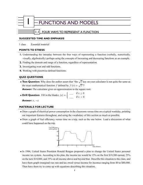
1 FUNCTIONS AND MODELS

1 FUNCTIONS AND MODELS
1.1 FOUR WAYS TO REPRESENT A FUNCTION
SUGGESTED TIME AND EMPHASIS
1 class Essential material
POINTS TO STRESS
1. Understanding the interplay between the four ways of representing a function (verbally, numerically,
visually, algebraically) perhaps using the concepts of increasing and decreasing functions as an example.
2. Finding the domain and range of a function, regardless of representation.
3. Investigating even and odd functions.
4. Working with piecewise defined functions.
QUIZ QUESTIONS
• Text Question: Why does the author assert that “the √ x key on your calculator is not quite the same as
the exact mathematical function f defined by f (x) = √ x”?
Answer: The calculator gives an approximation to the square root.
{ ___ if x ≥ 0
• Drill Question: Fill in the blanks: |x| =
___ if x < 0
Answer: x, −x
MATERIALS FOR LECTURE
• Draw a graph of electrical power consumption in the classroom versus time on a typical weekday, pointing
out important features throughout, and using the vocabulary of this section as much as possible.
• Draw a graph of fuel efficiency versus time on a trip, such as the one below. Lead a discussion of what
could have happened on the trip.
Fuel Efficiency
(miles/gallon)
30
20
10
0 1 2 3 Time (Hours)
• In 1984, United States President Ronald Reagan proposed a plan to change the United States personal
income tax system. According to his plan, the income tax would be 15% on the first $19,300 earned, 25%
on the next $18,800, and 35% on all income above and beyond that. Describe this situation to the class, and
have them graph (marginal) tax rate and tax owed versus income for incomes ranging from $0 to $80,000.
Then have them try to come up with equations describing this situation.
1

CHAPTER 1
FUNCTIONS AND MODELS
• In the year 2000, Presidential candidate Steve Forbes proposed a “flat tax” model: 0% on the first $36,000
and 17% on the rest. Have the students do the same analysis, and compare the two models. As an extension,
perhaps have the students look at a current tax table and draw similar graphs.
WORKSHOP/DISCUSSION
• Present graphs of even and odd functions, such as sin x, cosx + x 2 , and cos (sin x), and check with the
standard algebraic tests.
• Start with a table of values for a function f , such as the following:
x 0 1 2 3 4
f (x) 0 0.5 2 4.5 8
First, have the class describe the behavior of the function in words, trying to elicit the information that the
function is increasing, and that its rate of increase is also increasing. Then, have them try to extrapolate
the function in both directions, debating whether or not the function is always positive and increasing. Plot
the points and connect the dots, then have them try to concoct a formula (not necessarily expecting them
to succeed).
{ √ x if x is rational
• Discuss the domain and range of a function such as f (x) =
0 if x is irrational
Also talk about why f is neither increasing nor decreasing for x > 0. Stress that when dealing with new
sorts of functions, it becomes important to know the precise mathematical definitions of such terms.
• Define “difference quotient” as done in the text. Define f (x) = x 3 ,andshowthat
f (a + h) − f (a)
= 3a 2 + 3ah + h 2 . This example both reviews algebra skills and foreshadows future
h
calculations.
GROUP WORK 1: Every Picture Tells a Story
Put the students in groups of four, and have them work on the exercise. If there are questions, encourage them
to ask each other before asking you. After going through the correct matching with them, have each group
tell their story to the class and see if it fits the remaining graph.
Answers: 1. (b) 2. (a) 3. (c) 4. The roast beef was cooked in the morning and put in the refrigerator
in the afternoon.
GROUP WORK 2: Finding a Formula
Make sure that the students know the equation of a circle with radius r, and that they remember the notation
for piecewise-defined functions. Split the students into groups of four. In each group, have half of the students
work on each problem first, and then have them check each other’s work. If the students find these problems
difficult, have them work together on each problem.
⎧
⎧
x + 4 if x ≤−2
⎪⎨ −x − 2 if x ≤−2
⎪⎨ 2 if−2 < x ≤ 0
Answers: 1. f (x) = x + 2 if−2 < x ≤ 0 2. g(x) = √
⎪⎩
4 − x 2 if 0 < x ≤ 2
2 if x > 0
⎪⎩
x − 2 if x > 2
2

SECTION 1.1
FOUR WAYS TO REPRESENT A FUNCTION
HOMEWORK PROBLEMS
Core Exercises: 2, 10, 18, 19, 21, 24, 28, 51, 61
Sample Assignment: 2, 4, 6, 10, 13, 16, 18, 19, 20, 21, 24, 28, 51, 57, 61
Exercise D A N G
2 ×
4 × ×
6 ×
10 × ×
13 ×
16 × ×
18 ×
19 × ×
Exercise D A N G
20 × ×
21 ×
24 ×
28 ×
51 ×
57 ×
61 ×
3

GROUP WORK 1, SECTION 1.1
Every Picture Tells a Story
One of the skills you will be learning in this course is the ability to take a description of a real-world occurrence,
and translate it into mathematics. Conversely, given a mathematical description of a phenomenon, you
will learn how to describe what is happening in plain language. Here follow four graphs of temperature versus
time and three stories. Match the stories with the graphs. When finished, write a similar story that would
correspond to the final graph.
T
T
Graph 1
t
Graph 2
t
T
T
t
t
Graph 3
Graph 4
(a) I took my roast beef out of the freezer at noon, and left it on the counter to thaw. Then I cooked it in the
oven when I got home.
(b) I took my roast beef out of the freezer this morning, and left it on the counter to thaw. Then I cooked it in
the oven when I got home.
(c) I took my roast beef out of the freezer this morning, and left it on the counter to thaw. I forgot about it,
and went out for Chinese food on my way home from work. I put it in the refrigerator when I finally got
home.
4

GROUP WORK 2, SECTION 1.1
Finding a Formula
Find formulas for the following functions:
1.
y
1
0
1
x
2.
y
1
0
r=2
1
x
5

1.2 MATHEMATICAL MODELS: A CATALOG OF ESSENTIAL FUNCTIONS
TRANSPARENCY AVAILABLE
#1 (Figure 12)
SUGGESTED TIME AND EMPHASIS
1 class Recommended material
POINTS TO STRESS
1. The modeling process: developing, analyzing, and interpreting a mathematical model.
2. Classes of functions: linear, power, rational, algebraic, trigonometric, exponential and transcendental
functions. Include the special characteristics of each class of functions.
QUIZ QUESTIONS
• Text Question: What is the difference between a power function x n with n = 3 and a cubic function?
Answer: A cubic function can have lower order terms, whereas a power function has just one term.
• Drill Question: Classify each function graphed below as a power function, root function, polynomial,
rational function, algebraic function, or trigonometric function. Explain your reasoning.
y
y
y
10
4
4
2
2
5
_2 _1 0 1 2 x
_2
_2 _1 1 2 x
_2
_5 _4 _3 _2 _1 0 1 2 3 4
_5
5
x
_4
Answer: Polynomial, trigonometric, trigonometric
_4
_10
MATERIALS FOR LECTURE
• Show that linear functions have constant differences in y-values for equally spaced x-values. This example
illustrates the point:
Linear function (difference=1.2)
x f (x)
−2 −2.0
0 −0.8
2 0.4
4 1.6
• Discuss the shape, symmetries, and general “flatness” near 0 of the power functions x n for various values
of n. Similarly discuss n√ x for n even and n odd. A blackline master is provided at the end of this section,
before the group work handouts.
• If Exercises 18–22 are to be assigned, Exercise 17 can be done in class (with part (c) being discussed in the
context of the technology the students have available). Attached is a guide to using a graphing calculator
6

SECTION 1.2
MATHEMATICAL MODELS: A CATALOG OF ESSENTIAL FUNCTIONS
to do regression analysis. The guide was specifically written for the TI-85, but students with various other
calculators may also find it helpful.
WORKSHOP/DISCUSSION
• Have the students graph 2 x ,sinx, sin2 x ,and2 sin x . Discuss why the latter two look the way that they
do, then discuss the relationship among the graphs of f (x) = 2 x , g (x) = (0.5) x , h (x) = 2 −x ,and
k (x) = 4 x .
• Figure 17 shows examples of a noncontinuous function and a nondifferentiable function, both expressible
as simple formulas. Discuss these curves with the students, trying to get them to describe the ideas of a
break in a graph and a cusp.
GROUP WORK 1: Rounding the Bases
On the board, review how to compute the percentage error when estimating π by 22 7
.(Answer:0.04%) Have
them work on the problem in groups. If a group finishes early, have them look at h(7) and h(10) to see how
fast the error grows. Exponential functions will be covered in more detail in Chapter 7.
Answers: 1. 17.811434627, 17, 4.56% 2. 220.08649875, 201, 8.67% 3. 45.4314240633, 32, 29.56%
GROUP WORK 2: The Small Shall Grow Large
If a group finishes early, ask them to similarly compare x 3 and x 4 .
Answers: 1. x 6 ≥ x 8 for −1 ≤ x ≤ 1 2. x 3 ≥ x 5 for −∞ < x ≤−1, 0 ≤ x ≤ 1 3. x 3 ≥ x 105 for
−∞ < x ≤−1, 0 ≤ x ≤ 1. If the exponents are both even, the answer is the same as for Problem 1, if the
exponents are both odd, the answer is the same as for Problem 2.
GROUP WORK 3: Fun with Fourier
This activity should be given before Fourier series are discussed in class. This activity will get students
looking at combinations of sine curves, while at the same time foreshadowing the concepts of infinite series
and Fourier series.
Answers:
1. No
2. S (x) =
{ 1 if−2π ≤ x < −π or 0 ≤ x < π
−1 if−π ≤ x < 0orπ ≤ x ≤ 2π
4
π
3. Answers will vary. sin x has the advantage of being an odd function, like the square wave. Some
4
students will believe that
π
cos x has the same y-intercept as the square wave. This provides a good
opportunity to point out that the square wave has no y-intercept — what happens just to the right of x = 0
is different from what happens just to the left of x = 0.
7

4.
)
4
π
(sin x + 1 3 sin 3x + 1 5 sin 5x
CHAPTER 1
FUNCTIONS AND MODELS
y
1
_6 _4 _2 0 2 4 6 x
5.
(
4 sin 3x
sin x +
π
3
+
sin 5x
5
+
sin 7x
7
+
sin 9x
9
+
_1
sin 11x
11
+
sin 13x
13
+
sin 15x
15
+
sin 17x
17
+
)
sin 19x
19
y
1
_2¹
_¹
¹ 2¹
x
_1
6. y
¹/2
_2¹ _¹ 0
_¹/2
¹ 2¹
x
USING A GRAPHING CALCULATOR TO DO REGRESSION ANALYSIS
The following instructions assume the use of a TI-85 calculator.
• Under the STAT menu select EDIT.
• Choose desired lists for x-andy-coordinates.
• Enter the x-andy-coordinates of the data.
• In graph mode, set approximate ranges so points can be viewed. Erase or deselect all functions.
• In default window, choose a regression model:
• ExpR (Exponential regression)
• LinR (Linear regression)
• LnR (Logarithmic regression)
• P2Reg (Quadratic regression)
• P3Reg (Cubic regression)
• P4Reg (Quartic regression)
• Under STAT mode, select DRAW.
• Select SCAT to plot data points.
• Select DRREG to plot the regression model.
• Move cursor along regression plot to get approximations for interpolation.
8

SECTION 1.2
MATHEMATICAL MODELS: A CATALOG OF ESSENTIAL FUNCTIONS
HOMEWORK PROBLEMS
Core Exercises: 4, 8, 15, 18, 21, 23
Sample Assignment: 4, 8, 9, 10, 12, 15, 18, 19, 21, 23, 25
Exercise D A N G
4 × ×
8 × ×
9 ×
10 × ×
12 × ×
15 × ×
18 × × ×
19 × ×
21 × × ×
23 × × × ×
25 × ×
9

CHAPTER 1
FUNCTIONS AND MODELS
y
1
y
1
y
1
0
x
1
x
0 1 x
0 1
x 2 x 3
x
y
1
y
1
y
1
0 1 x
0 1 x
0 1
x 4 x 5 x 6
x
y
1
y
1
y
1
0
x
1
x
0 1 x
0 1
√ x 3√ x
x
y
1
y
1
y
1
0 1 x
0 1 x
0 1
4√ x 5√ x 6√ x
x
10

GROUP WORK 1, SECTION 1.2
Rounding the Bases
1. For computational efficiency and speed, we often round off constants in equations. For example, consider
the linear function
f (x) = 3.137619523x + 2.123337012
In theory, it is very easy and quick to find f (1), f (2), f (3), f (4), and f (5). In practice, most people
doing this computation would probably substitute
f (x) = 3x + 2
unless a very accurate answer is called for. For example, compute f (5) both ways to see the difference.
The actual value of f (5):
The “rounding” estimate:
The percentage error:
__________
__________
__________
2. Now consider
g (x) = 1.12755319x 3 + 3.125694x 2 + 1
Again, one is tempted to substitute g (x) = x 3 + 3x 2 + 1.
The actual value of g (5):
The “rounding” estimate:
The percentage error:
__________
__________
__________
3. It turns out to be very dangerous to similarly round off exponential functions, due to the nature of their
growth. For example, let’s look at the function
h (x) = (2.145217198123) x
One may be tempted to substitute h (x) = 2 x for this one. Once again, look at the difference between
these two functions.
The actual value of h (5): __________
The “rounding” estimate:
The percentage error:
__________
__________
11

GROUP WORK 2, SECTION 1.2
The Small Shall Grow Large
1. For what values of x is x 6 ≥ x 8 ? For what values is x 6 ≤ x 8 ?
2. For what values of x is x 3 ≥ x 5 ?
3. For what values of x is x 3 ≥ x 105 ? Can you generalize your results?
12

GROUP WORK 3, SECTION 1.2
Foreshadowing Fourier
The following function S (x) is called a “square wave”.
y
1
_2¹ _¹ 0
_1
¹ 2¹
x
1. Can you find a function on your calculator which has the given graph?
2. Write a formula that has this graph for −2π ≤ x ≤ 2π.
3. Which of the functions sin x and cos x gives a better approximation to S (x)?
4. Select the function from among the following which gives the best approximation to the square wave:
sin x,sinx + sin 3x,sinx + 1 2 sin 3x,sinx + 1 3 sin 3x, and sin x + 1 4
sin 3x.
5. Find the integer n which makes f (x) = sin x + 1 3 sin 3x + n 1 sin 5x the best possible approximation to the
square wave.
13

Foreshadowing Fourier
6. A Fourier approximation of a function is an approximation of the form
F (x) = a 0 + a 1 cos x + b 1 sin x + a 2 cos 2x + b 2 sin 2x +···+a n cos nx + b n sin nx
You have just discovered the Fourier approximation to S (x) with three terms. Find the Fourier
approximation to S (x) with ten terms, and sketch its graph.
7. The following expressions are Fourier approximations to a different function, T (x):
T (x) ≈ sin x
T (x) ≈ sin x − 1 2
sin 2x
T (x) ≈ sin x − 1 2 sin 2x + 1 3
sin 3x
T (x) ≈ sin x − 1 2 sin 2x + 1 3 sin 3x − 1 4
sin 4x
T (x) ≈ sin x − 1 2 sin 2x + 1 3 sin 3x − 1 4 sin 4x + 1 5
sin 5x
Sketch T (x).
14

1.3 NEW FUNCTIONS FROM OLD FUNCTIONS
SUGGESTED TIME AND EMPHASIS
1 class Essential material
POINTS TO STRESS
1. The mechanics and geometry of transforming functions.
2. The mechanics and geometry of adding, subtracting, multiplying, and dividing functions.
3. The mechanics and geometry of composing functions.
QUIZ QUESTIONS
( )
• Text Question: Label the following graphs: f (x), 1 2 f (x) , f 12
x .
y
1
y
1
y
1
0 2 x
0 2 x
0 2 x
( )
Answer: 1 2 f (x), f 12
x , f (x)
• Drill Question: How can we construct the graph of y = | f (x)| from the graph of y = f (x)? Explain
in words, and demonstrate with the graph of y = x 2 − 4.
Answer: We leave the positive values of f (x) alone, and reflect the negative values about the x-axis.
y
y
2
2
0
1 x
0
1 x
y = x 2 − 4
15
y = ∣ ∣x 2 − 4 ∣ ∣

CHAPTER 1
FUNCTIONS AND MODELS
MATERIALS FOR LECTURE
• Using f (x) = x sin x, explore graphs of f (x + 2), f (x) + 2, − f (x), f (−x), | f (x)|. Note why
f (−x) = f (x).
• Graph f (x) = sin (√ x ) and g (x) = √ sin x. Draw the relevant “arrow diagrams” and then write them in
the forms l ◦ k and k ◦ l. Then discuss reasons for the differences in their graphs.
Answer: See the text for sample arrow diagrams. f is a sine function whose argument grows larger more
and more slowly as we move away from the origin. g is a root function whose argument oscillates, causing
g to oscillate as well.
WORKSHOP/DISCUSSION
• Using f (x) = 1/x 2 and g (x) = cos x, compute the domains of f + g, f/g, g/f , f ◦ g, andg ◦ f ,and
the range of g ◦ f . Pay particular attention to the domain of g/f , as many students will think it is R.
• Do the following problem with the students:
y
y=f(x)
1
0
1
x
From the graph of y = f (x) =−x 2 + 2 shown above, compute f ◦ f at x =−1, 0, and 1. First do it
graphically (as in Exercises 59 and 60), then algebraically.
• TEC Using TEC or a graphing calculator, have the students graph the following functions, where
f (x) = x + x 2 , first guessing what each graph will look like.
1. f (2x) 4. −2 f (x) 7. f (x) + 2
(
2. f 12
x)
5. f (x − 2) 8. 2 f (2x)
(
3. 2 f (x) 6. f (x) − 2 9. 2 f 12
x)
GROUP WORK 1: Which is the Original?
Answers: 1. 2 f (x + 2),2f (x), f (2x), f (x + 2), f (x) 2. 2 f (x), f (x), f (x + 2), f (2x),2f (x + 2)
GROUP WORK 2: Label Label Label, I Made It Out of Clay
Some of these transformations were not covered directly in the book. If the students are urged not to give
up, and to use the process of elimination and testing individual points, they should be able to complete this
activity.
Answers: 1. (d) 2. (a) 3. (f) 4. (e) 5. (i) 6. (j) 7. (b) 8. (c) 9. (g) 10. (h)
16

SECTION 1.3
NEW FUNCTIONS FROM OLD FUNCTIONS
GROUP WORK 3: It’s More Fun to Compute
Each group gets one copy of the graph. During each round, one representative from each group stands,
and one of the questions below is asked. The representatives write their answer down, and all display their
answers at the same time. Each representative has the choice of consulting with their group or not. A correct
solo answer is worth two points, and a correct answer after a consult is worth one point.
Answers: 1. 0 2. 0 3. 1 4. 5 5. 1 6. 1 7. 1 8. 0 9. 2 10. 1 11. 1 12. 1
HOMEWORK PROBLEMS
Core Exercises: 1, 5, 10, 29, 31, 39, 50, 51, 54, 60
Sample Assignment: 1, 5, 6, 10, 17, 26, 28, 29, 31, 39, 42, 50, 51, 54, 56, 57, 59, 60, 62, 63
Exercise D A N G
1 ×
5 ×
6 × ×
10 ×
17 ×
26 × ×
28 × ×
29 ×
31 ×
39 ×
Exercise D A N G
42 ×
50 × ×
51 × ×
54 × ×
56 × ×
57 × × ×
59 ×
60 × ×
62 ×
63 ×
17

GROUP WORK 1, SECTION 1.3
Which is the Original?
Below are five graphs. One is the graph of a function f (x) and the others include the graphs of 2 f (x),
f (2x), f (x + 2),and2f (x + 2). Determine which is the graph of f (x) and match the other functions with
their graphs.
1.
y
y
y
1
1
1
0 1 x
0 1 x
0 1 x
Graph 1 Graph 2 Graph 3
y
y
1
1
0
1 x
0
1 x
2.
y
Graph 4
y
Graph 5
y
1
1
1
0 1 x
0 1 x
0 1 x
Graph 1 Graph 2 Graph 3
y
y
1
1
0
1 x
0
1 x
Graph 4
Graph 5
18

This is a graph of the function f (x):
GROUP WORK 2, SECTION 1.3
Label Label Label, I Made it Out of Clay
y
5
0
2
x
Give each graph below the correct label from the following:
(a) f (x + 3) (b) f (x − 3) (c) f (2x) (d) 2 f (x) (e) | f (x)|
(f) f (|x|) (g) 2 f (x) − 1 (h) f (2x) + 2 (i) f (x) − x (j) 1/f (x)
y
y
y
y
5
5
5
5
0 2
x
0 2
x
0 2
x
0 2
x
Graph 1 Graph 2 Graph 3 Graph 4
y
y
y
y
5
5
5
5
0 2
x
0 2
x
0 2
x
0 2
x
Graph 5 Graph 6 Graph 7 Graph 8
y
y
5
5
0 2
x
0 2
x
Graph 9 Graph 10
19

Using the graph below, find the following quantities.
GROUP WORK 3, SECTION 1.3
It’s More Fun to Compute
1. ( f ◦ g)(5) 5. (g ◦ g)(5) 9. (g ◦ f )(1)
2. (g ◦ f )(5) 6. (g ◦ g)(−3) 10. ( f ◦ f ◦ g)(4)
3. ( f ◦ g)(0) 7. (g ◦ g)(−1) 11. (g ◦ f ◦ f )(4)
4. ( f ◦ f )(5) 8. ( f ◦ g)(1) 12. ( f ◦ g ◦ f )(4)
y
5
4
3
f
2
1
g
0
_5 _4 _3 _2 _1 1 2 3 4 5
x
_1
_2
_3
_4
_5
20

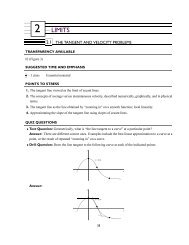
1.4 GRAPHING CALCULATORS AND COMPUTERS
SUGGESTED TIME AND EMPHASIS
1
2
–1 class Optional material (If unassigned, students should be encouraged to read this self-contained
section on their own.)
POINTS TO STRESS
1. When graphing an arbitrary function, some viewing windows are more appropriate than others, depending
on the context of the inquiry and some analysis of the actual equation.
2. Some functions don’t have any single viewing window that will give all the important details of the
function.
3. One can use zoom and trace features to obtain estimates of solutions to difficult algebraic equations.
4. Graphing calculators can give misleading or wrong answers.
QUIZ QUESTIONS
• Text Question: Why is it true that “The solutions of the equation cos x = x are the x-coordinates of the
points of intersection of the curves y = cos x and y = x”?
Answer: If y = cos x and y = x,wecanusesubstitutiontosetx = y = cos x.
• Drill Question: Find all solutions of the equation x 3 − 10x 2 − 4 = 0 correct to at least two decimal
places.
Answer: x ≈ 10.0397
MATERIALS FOR LECTURE
• Caution students to take care when using their calculators, particularly when choosing a viewing window.
The following are features of a function that are difficult to determine solely from computer graphics:
• End behavior. For example, f (x) = log 10 x
100 sin x
• Certain asymptotes, such as oblique asymptotes. For example, f (x) = 3x + 2 + 5√ , x > 2 x
• The effects of parameters. For example, f (x) = sin ( Ax b)
• Hidden roots. For example, the roots of f (x) = x 4 − 0.001x
• Domains and ranges. For example, the domain of √ sin (x + cos x), the range of sin x
x
• Have the class experiment with f (x) = cos
(x + 1 )
x 2 near x = 0, and also for large values of x.
• Attempt to graph f (x) = √ x − 2 √ x − 4, and to find its domain. Certain packages or calculators (like
the TI-89, Maple, and Mathematica) will graph it incorrectly, with domain (−∞, 2) ∪ (4, ∞). Discuss
why some software makes this error.
Answer: For x < 2, each of these algebra packages converts both multiplicands into imaginary numbers,
multiplies them, and then converts the product back into a real number. This process is invalid in the
context of real-valued functions.
21

CHAPTER 1
FUNCTIONS AND MODELS
• Demonstrate the use of a calculator as an investigative tool (for example, to explore a family of functions
like f (x) = Qx + cos x by graphing with Q = 0.5, 0.75, 0.95,1,and1.1). Discuss the meaning of
“parameter” using Q as an example. Be sure to note that when Q < 1, the function has “peaks and
valleys” (local maxima and minima) and when Q > 1 the function is always increasing.
Answer:
y
y
y
1
1
1
0
2 x
0
2 x
0
2 x
Q = 0.5
y
Q = 0.75
y
Q = 0.95
1
1
0
2 x
0
2 x
Q = 1
Q = 1.1
WORKSHOP/DISCUSSION
• Pose the question, “What happens to cos x − 1 as x gets close to zero?” Show how the strategy of
x
substituting x = 0 fails. Investigate this question numerically, and then by graphing. Follow up with the
function cos x − 1
x 2 .
Answer: As x gets close to zero, the value of cos x − 1 gets close to zero. as x gets close to zero, the
x
value of cos x − 1
x 2 gets close to − 1 2 .
• Have the students try to figure out what the graph of f (x) = [x + 0.05 cos (20x)] 2 looks like near x = 0
by experimenting with viewing windows. Then have them try to explain why their picture makes sense.
• Have the students first determine where f (x) = x 3 − 50x 2 is larger than x 2 .Pointoutthatitiseasierto
use some algebra to solve this problem than to use a calculator
Answer: x > 51
• Have the students first guess the shape of f (x) = √ sin x, and then graph it. Ask how they should have
known it would be periodic.
22

SECTION 1.4
GRAPHING CALCULATORS AND COMPUTERS
GROUP WORK 1: Short- and Long-Term Behavior
Before handing this exercise out, show what is meant by “long-term behavior”.
Part of the idea of this exercise is getting the students to explore and play with functions (even unfamiliar ones)
on their calculators. Encourage them to try varying the functions on the worksheet, and see what happens.
Answers: 1. (a) f (x) →∞as x →∞ (b) x = 0, x ≈−0.877 2. (a) g (x) →∞as x →∞(g is
asymptotic to y = 6x) (b) None 3. (a) h (x) →∞as x →∞ (b) x = 0, ± √ 3 4. (a) j (x) → 1as
x →∞ (b) None 5. (a) k (x) →−∞as x →∞ (b) x ≈ 0.4027, 0.9952, 1.923 6. (a) l (x) →−∞
as x →∞ (b) x = 0
GROUP WORK 2: Just Two Solutions
This is an extension of Exercise 24. It is a difficult exercise, and the students may require some guidance.
Before handing out the hint sheet, have the students try to solve this problem on their own: “Consider the
equation cos x = mx. Find a value of m such that this equation has exactly two solutions.” After they have
worked on the problem, and are clear on what they are trying to find, hand out the hint sheet. Don’t let them
hang too long! Conclude by discussing how the line y = mx that yields exactly two solutions is called tangent
to the curve y = cos x. Explain that soon we will learn how to find the equation of such a line. This is a
good example to bring back once they have covered derivatives of trigonometric functions in Section 3.5.
At that point, they will wind up having to solve the equation x =−cot x. Revisit the problem again after
covering Newton’s method in Section 4.9, at which point they will finally have a way of approximating m to
any desired accuracy.
Answers:1.,3.,7.
y 1 2
1
3
4
5
2. 1, 3
5. m ≈±0.33651
6. Symmetry
_8 _6 _4 _2 0 2 4 6 8 x
_1
HOMEWORK PROBLEMS
Core Exercises: 5, 8, 19, 22, 26, 29
Sample Assignment: 5, 8, 15, 18, 19, 22, 24, 26, 27, 29, 35
Exercise D A N G
5 ×
8 ×
15 ×
18 ×
19 ×
22 × ×
Exercise D A N G
24 ×
26 × ×
27 × ×
29 × ×
35 ×
23

GROUP WORK 1, SECTION 1.4
Short- and Long-Term Behavior
For each of the following functions, (a) describe the long term behavior of the function, and (b) locate the
zeros,ifany.
1. f (x) = sin x + x 2
2. g (x) = 6x + 1 x = 6x2 + 1
x
3. h (x) = x3 − 3x
x + 7
4. j (x) = 2 −1/x6
5. k (x) = x 5 − 2x 4 − x 2 + 3x − 1.01 x
6. l (x) = Qx + sin x for Q = 0.32, 0.9, and 1.1 What are the differences among these three functions?
24

GROUP WORK 2, SECTION 1.4
Just Two Solutions (Hint Sheet)
Problem: Find a value of m such that the equation cos x = mx has exactly two solutions.
1. Very carefully, draw graphs of the following three functions below: y = cos x, y = x, y = 1 5 x.
y
1
_8 _6 _4 _2
2
4 6 8
x
_1
2. From the graphs, determine how many solutions the equation has for m = 1 and for m = 1 5 .
3. Add a sketch of y = mx onto your picture for Problem 1, where m is chosen so that the equation
cos x = mx has exactly two solutions. You can do this without actually computing m.
4. Use your sketch to estimate the correct value of m.
5. Now use your graphing calculator to refine your guess. Try to get an answer correct to three decimal
places.
6. Why is it true that the value −m will also give exactly two solutions to cos x = mx?
7. Is it possible to find a value of m such that cos x = mx has exactly three solutions? Four? n? Explain
your answer by sketching y = cos x and y = mx for the relevant values of m.
25

1 SAMPLE EXAM
Problems marked with an asterisk (*) are particularly challenging and should be given careful consideration.
1. The graph below shows the temperature of a room during a summer day as a function of time, starting at
midnight.
(a) Evaluate f (noon) and f (6 P.M.). State the range of f .
6 12
18
24 t (h)
(b) Where is f increasing? Decreasing?
(c) Give a possible explanation for what happened at noon.
(d) Give a possible explanation why f attains its minimum value at 6 A.M.
2. A proposed new grain silo consists of a cylinder of height h and radius r, capped by a hemisphere.
Express its volume as a function of h and r.
26

CHAPTER 1
SAMPLE EXAM
3. The Slopps R○ trading card company has decided to put out its best line of trading cards ever: The “Famous
Mathematicians” Series. Each pack of cards contains eight famous mathematicians, a mathematical
puzzle, and a mathematics sticker. Naturally, you want a complete set, but you will have to buy a lot
of cards because the really good ones (like the Galois, Sylvester, Hesse, Newton, and Leibniz cards) are
very rare. Your local dealer will sell you an individual card, randomly selected, for 50 cents. Most people
are interested in buying the packs of 8 for $2.80. When you tell the dealer you want to buy a lot of them,
he offers to sell you a box (containing 10 packs) for $25, or a carton (containing 10 boxes) for $230.
Let c (x) be the (least) cost of buying x cards. Note that it is acceptable to buy more than x cards if it costs
less than buying exactly x cards.
(a) Explain why the cheapest way to buy 6 cards is to buy a pack of 8. What is c (6)?
(b) Sketchagraphofy = c (x) from x = 0tox = 24.
(c) Find a formula for c (x), valid for x = 80 to x = 90.
(d) If you wanted to buy 1005 cards, what is the least you would have to pay?
27

CHAPTER 1
FUNCTIONS AND MODELS
4. The following is a graph of y = f (x).
y
4
2
0
2 4 6 8 x
_2
_4
On the same axes, draw and label graphs of
(a) 2 f (x + 2)
(c)
f (2x)
y
8
(b) 1 2 f (−x) 2 4 6 8 x
y
8
y
8
6
6
6
4
4
4
2
2
2
_8
_6
_4
_2
0
2 4 6 8 x
_8
_6
_4
_2
0
_8
_6
_4
_2
0
2 4 6 8 x
_2
_2
_2
_4
_4
_4
_6
_6
_6
_8
_8
_8
(d) 2 f (2x − 2)
(e) f (2x) − 2
y
y
8
8
6
6
4
4
2
2
_8
_6
_4
_2
0
2 4 6 8 x
_8
_6
_4
_2
0
2 4 6 8 x
_2
_2
_4
_4
_6
_6
_8
_8
28

CHAPTER 1
SAMPLE EXAM
5. Use the given graphs of f and g to evaluate each expression, or explain why it is undefined.
(a) ( f ◦ g)(2)
(b) (g ◦ f )(2)
(c) ( f ◦ f )(2)
(d) (g ◦ g)(2)
(e) ( f + g)(2)
(f) ( f/g)(2)
29

CHAPTER 1
FUNCTIONS AND MODELS
6. Find a formula that describes the following function.
y
1
1
_2
_1
0 1 2
x
7. Let f (x) = 2.912345x 2 + 3.131579x − 0.099999
(a) To simplify approximation of f , write a quadratic function g (x) with integer coefficients that closely
models f (x) for −10 < x < 10.
(b) Compute g (4) and f (4) .
(c) Compute the error in using g (4) to approximate f (4) as a percentage of the correct answer f (4).
(d) For larger values of x (say x = 10 or x = 20), would g (x) be an overestimate or an underestimate of
f (x)? Justify your answer without computing specific values of f and g.
30

CHAPTER 1
SAMPLE EXAM
8. A manufacturer hires a mathematician to come up with a function f that models the cost C of producing
a alternative-music compact discs, where C is in thousands of dollars. The graph of f is given below.
(a) What does f (50,000) − f (49,999) represent?
(b) For what value or range of values is the cost per disc the least?
(c) Give a possible explanation for the sudden increase in the curve’s slope at the end.
31

1 SAMPLE EXAM SOLUTIONS
1. Approximate answers are acceptable for this problem.
(a) f (noon) = 87 ◦ , f (6 P.M.) = 67 ◦ , range of f is [53, 87].
(b) f is increasing on (6, 12) and (20, 22); f is decreasing on (0, 6), (12, 20) and (22, 24).
(c) Possible explanations for the drop in temperature at noon are a sudden thundershower, or an air conditioner
being turned on.
(d) A possible explanation for f attaining its minimum value at 6 A.M. is that this is just before sunrise.
2. The total volume is the volume of a cylinder of height and radius r plus the volume of a hemisphere of
radius r,thatis,V = πr 2 h + 2 3 πr3 .
3. (a) If we buy 8 cards for $2.80, then this costs less than buying 6 individual cards at $0.50 apiece. Hence,
C (6) = $2.80.
(b) c
10
5
0 3 6 9 12 15 18 21 24 x
⎧
⎨ 25 + 0.5 (x − 80) if 80 ≤ x ≤ 85
(c) c (x) = 27.8 if86 ≤ x ≤ 88
⎩
27.8 + 0.5 (x − 88) if 89 ≤ x ≤ 90
(d) To buy 1005 cards, the best deal is to buy one carton (800 cards), two boxes (160 cards), five packs
(40 cards) and five individual cards. The total cost would be
230 + 2 (25) + 5 (2.80) + 5 (0.50) = $296.50
4. (a)
y
8
(b)
y
1
4
_6 _4 _2 0 x
_2
0
2 4 x
_4
_4
_8
32

CHAPTER 1
SAMPLE EXAM SOLUTIONS
(c)
y
(d)
y
(e)
y
2
4
0
2 4 x
0
1 2 x
0
2 4 x
_4
_2
_4
_8
_8
5. (a) ( f ◦ g)(2) = f (0) = 1
(b) (g ◦ f )(2) = g (3) = 1
(c) ( f ◦ f )(2) = f (3) = 4
(d) (g ◦ g)(2) = g (0) = 4
(e) ( f + g)(2) = f (2) + g (2) = 3 + 0 = 3
( ) f
(f) (2) is undefined because g (2) = 0.
g
⎧
⎨ √
−x − 1 if x < −1
6. f (x) = 1 − x
⎩
2 if −1 ≤ x ≤ 1
−x + 1 if x > 1
7. (a) g (x) = 3x 2 + 3x
(b) g (4) = 60, f (4) = 59.023837
(c) The percentage error in using g (4) as an approximation for f (4) is 100
∣
f (4) − g (4)
g (4)
∣ = 1.63%.
(d) For larger values of x, g (x) is an overestimate of f (x) because the coefficient of the dominant term
(x 2 )islarger.
8. (a) f (50, 000) − f (49, 999) represents the cost of producing the 50,000th disc.
(b) The cost per disc is cheapest for 30, 000 < a < 40, 000. This is where the slope of f is the smallest.
(c) One possible explanation for the sudden increase in the curve’s slope is scarcity of materials.
33