Chapter 4 Numerical Differentiation And Integration

Chapter 4
Numerical Differentiation And
Integration
Divided the interval [a,b],
a = x 0 < x 1 < ... < x n−1 < x n = b,
x k = a + kh, h = b − a
n
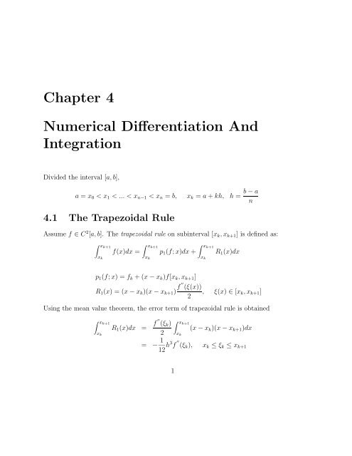
4.1 The Trapezoidal Rule
Assume f ∈ C 2 [a,b]. The trapezoidal rule on subinterval [x k ,x k+1 ] is defined as:
∫ xk+1
∫ xk+1
f(x)dx = p 1 (f;x)dx +
x k x k
∫ xk+1
x k
R 1 (x)dx
p 1 (f;x) = f k + (x − x k )f[x k ,x k+1 ]
R 1 (x) = (x − x k )(x − x k+1 ) f ′′ (ξ(x))
, ξ(x) ∈ [x k ,x k+1 ]
2
Using the mean value theorem, the error term of trapezoidal rule is obtained
∫ xk+1
x k
R 1 (x)dx = f ′′ (ξ k )
2
∫ xk+1
x k
(x − x k )(x − x k+1 )dx
= − 1 12 h3 f ′′ (ξ k ), x k ≤ ξ k ≤ x k+1
1

Then the trapezoidal rule is rewritten as:
∫ xk+1
The composite trapezoidal rule
∫ b
a
f(x)dx =
x k
f(x)dx = h 2 (f k + f k+1 ) − 1 12 h3 f ′′ (ξ k )
n−1 ∑
k=0
∫ xk+1
x k
f(x)dx
= h 2 (f 0 + 2f 1 + ... + 2f n−1 + f n ) − 1 n−1 ∑
12 h3
The error term of composite trapezoidal integration rule is
En T (f) = − 1 n−1 ∑
12 h3 f ′′ (ξ k ) = − 1 [ 1
12 h2 (b − a)
n
k=0
= − 1 12 h2 (b − a)f ′′ (ξ)
n−1 ∑
k=0
k=0
f ′′ (ξ k )
f ′′ (ξ k )
]
4.2 Simpson’s Rule
f ′′ (ξ) = maxf ′′ (ξ k ), a ≤ ξ ≤ b.
Assume f ∈ C 4 [a,b]. The Simpson’s rule on subinterval [x k ,x k+2 ] is defined as:
∫ xk+2
∫ xk+2
f(x)dx = p 2 (f;x)dx +
x k x k
∫ xk+2
x k
R 2 (x)dx
p 2 (f;x) = f k + (x − x k )f[x k ,x k+1 ] + (x − x k )(x − x k+1 )f[x k ,x k+1 ,x k+2 ]
R 2 (x) = (x − x k )(x − x k+1 )(x − x k+2 )f[x k ,x k+1 ,x k+2 ,x]
Note that, since (x − x k )(x − x k+1 )(x − x k+2 ) changes sign at x = x ± k+1 , it can not use
the mean value theorem to obtain the error term, so define
∫ x
w(x) = (t − x k )(t − x k+1 )(t − x k+2 )dt
x k
w ′ (x) = (x − x k )(x − x k+1 )(x − x k+2 )
2

Then w(x k ) = w(x k+2 ) = 0 and w(x) > 0 for x k < x < x k+2 . Therefore, the error term
is obtained by integral by part and the mean value theorem
∫ xk+2
x k
R 2 (x)dx =
= −
∫ xk+2
x k
∫ xk+2
x k
w ′ (x)f[x k ,x k+1 ,x k+2 ,x]dx
w(x)f[x k ,x k+1 ,x k+2 ,x,x]dx
= −f[x k ,x k+1 ,x k+2 ,ξ,ξ]
= − 1 [ ] 4
24 f(4) (ξ k )
15 h5
∫ xk+2
x k
w(x)dx
∫ xk+2
x k
f(x)dx = h 3 (f k + 4f k+1 + f k+2 ) − 1 90 h5 f (4) (ξ k ), x k < ξ k < x k+2
The composite Simpson’s rule for even n
∫ b
f(x)dx = h 3 (f 0 + 4f 1 + 2f 2 + 4f 3 + 2f 4 + ... + 4f n−1 + f n )
a
− 1
180 h4 (b − a)f (4) (ξ).
Note that the Simpson’s rule is exact for polynomial of degree ≤ 3.
4.3 Newton-Cotes Integration Formulas
∫ b
∫ b n∑
n∑
I n (f) = p n (f;x)dx = l j,n (x)f(x j ) = w j,n f(x j )
a
a
j=0
j=0
w j,n =
∫ b
a
l j,n (x),
j = 0, 1,...,n
n = 1 I 1 = h [f(a) + f(b)] −h3
2
12 f ′′ (ξ)
n = 2 I 2 = h [f(a) + 4f(a + h) + f(b)] −h5
3
90 f(4) (ξ)
n = 3 I 3 = 3h 8
[f(a) + 3f(a + h) + 3f(a + 2h) + f(b)] −3h5
80 f(4) (ξ)
3

Theorem 4.1 (a) For n even, assume f(x) ∈ C n+2 [a,b]. Then
I(f) − I n (f) = C n h n+3 f (n+2) (η),
C n =
η ∈ [a,b]
∫
1 n
µ 2 (µ − 1)...(µ − n)dµ
(n + 2)! 0
(b) For n odd, assume f(x) ∈ C n+1 [a,b]. Then
proof :
I(f) − I n (f) = C n h n+2 f (n+1) (η),
C n =
E n (f) = I(f) − I n (f) =
η ∈ [a,b]
∫
1 n
µ(µ − 1)...(µ − n)dµ
(n + 1)! 0
∫ b
a
(x − x 0 )(x − x 1 )...(x − x n )f[x 0 ,x 1 ,...,x n ,x]dx
If n odd then (x − x 0 )(x − x 1 )...(x −x n ) is unchange sign on [a,b]. Using the mean value
theorem we obtain the (b) easily. If n even, define
w(x) =
∫ x
a
(t − x 0 )(t − x 1 )...(t − x n )dt, w ′ (x) = (x − x 0 )(x − x 1 )...(x − x n ).
Then w(a) = w(b) = 0 and w(x) > 0 for x ∈ [a,b]. Using the integral by part and the
mean value theorem we obtain the error term
E n (f) =
∫ b
a
w ′ (x)f[x 0 ,x 1 ,...,x n ,x]dx = −
= −f[x 0 ,x 1 ,...,x n ,ξ,ξ]
= − f(n+2) (η)
(n + 2)!
∫ b
a
w(x)dx =
∫ b ∫ x
a
a
∫ b ∫ b
a t
∫ xn
This completes the proof of theorem.
∫ b
a
w(x)dx,
∫ b
a
w(x)f[x 0 ,x 1 ,...,x n ,x,x]dx
a ≤ ξ ≤ b
(t − x 0 )(t − x 1 )...(t − x n )dtdx
(t − x 0 )(t − x 1 )...(t − x n )dxdt
= (t − x 0 )(t − x 1 )...(t − x n )(x n − t)dt
x 0
∫ n
= −h n+3 µ(µ − 1)...(µ − n) 2 dµ
0
∫ n
= −h n+3 µ 2 (µ − 1)...(µ − n)dµ
0
4

4.4 The Midpoint Rule
Using Taylor’s expansion for f(x) ∈ C 2 [a,b] at c = (b + a)/2
∫ b
a
f(x) = f(c) + f ′ (c)(x − c) + f ′′ (η)
(x − c) 2 , a ≤ η ≤ b
2
f(x)dx =
∫ b
a
f(c)dx +
∫ b
a
f ′ (c)(x − c)dx +
(b − a)3
= (b − a)f(c) + 0 + f ′′ (η)
24
Then we obtain the midpoint integration formula
∫ b
a
f(x)dx = (b − a)f( b + a
2
(b − a)3
) + f ′′ (η),
24
∫ b
a
f ′′ (η)
(x − c) 2 dx
2
η ∈ [a,b]
For the composite midpoint rule define x j = a + (j − 1 )h, j = 1, 2,...,n, the midpoints of
2
[a + (j − 1)h,a + jh]. Then
∫ b
a
f(x)dx = h[f 1 + f 2 + ... + f n ] +
(b − a)h2
f ′′ (η),
24
η ∈ [a,b]
4.5 Gauss-Legendre Quadrature
The generality integration formulas
n∑
I n (f) = w j,n f(x j,n ) =
.
j=1
∫ b
a
w(x)f(x)dx = I(f) (4.5.1)
The weight function w(x) is assumed to be nonnegative and integrable on [a,b]. The
special case w(x) = 1,
∫ 1
f(x)dx . n∑
= w j f(x j )
−1
j=1
The weight {w j } and nodes {x j } are to be determined to make the error
∫ 1
n∑
E n (f) = f(x)dx − w j f(x j )
−1
j=1
equal zero for as high a degree polynomial f(x) as possible. Note that E n (f) = 0 for
every polynomial of degree ≤ m if and only if E n (x i ) = 0, i = 0, 1,...,m.
5

(1) n=1. Since there are two parameters w 1 and x 1 , we consider
E n (1) = 0, E n (x) = 0
∫ 1
−1
1dx − w 1 = 0,
∫ 1
−1
xdx − w 1 x 1 = 0
This implies w 1 = 2 and x 1 = 0. Thus the formula is the midpoint rule,
∫ 1
f(x)dx = . 2f(0)
−1
(2) n=2. There are four parameters w 1 , w 2 , x 1 , x 2 and thus we put four constraints on
these parameters:
E n (x i ) =
∫ 1
−1
x i dx − [w 1 x i 1 + w 2 x i 2] = 0, i = 0, 1, 2, 3
These lead to the unique formula,
∫ 1
f(x)dx = . f(− √ 3/3) + f( √ 3/3)
−1
(3) For a general n there are 2n free parameters {x i } and {w i }. The equations to be
solved are
E n (x i ) = 0, i = 0, 1, 2,..., 2n − 1
These are nonlinear equations, and their solvability is not at all obvious.
The quadrature formula (4.5.1) has degree of exactness d if E n (f) = 0 for all f ∈ P d .
We call (4.5.1) interpolatory if it has degree of exactness d = n − 1. The interpolatory
formula is precisely for which
n∑
∫ b
w j f(x j ) = p n−1 (f;x 1 ,...,x n ;x)w(x)dx
j=1
a
n∑
n∏ x − x k
p n−1 (x) = l j (x)f(x j ), l j (x) =
j=1
k=1,k≠j
x j − x k
w j =
∫ b
a
l j (x)w(x)dx,
j = 1, 2,...,n.
6

Theorem 4.2 Given an integer k with 0 ≤ k ≤ n the quadrature formula (4.5.1) has
degree of exactness d = n−1+k if and only if both of the following conditions are satisfied
(a) The formula (4.5.1) is interpolatory.
(b) The node polynomial ω n (x) = ∏ n
j=1 (x − x j ) satisfies
∫ b
a
ω n (x)p(x)w(x)dx = 0,
∀ p ∈ P k−1
proof : (⇒) Since d = n − 1 + k ≥ n − 1, condition (a) is trivial. For any p(x) ∈ P k−1 ,
ω n (x)p(x) ∈ P n−1+k , hence
∫ b
n∑
ω n (x)p(x)w(x)dx = w j ω n (x j )p(x j ) = 0
a
j=1
since ω n (x j ) = 0, for j = 1, 2,...,n.
(⇐) Given any p(x) ∈ P n−1+k divide it by ω n (x), so that
p(x) = q(x)ω n (x) + r(x),
q ∈ P k−1 , r ∈ P n−1
∫ b
a
p(x)w(x)dx =
∫ b
a
q(x)ω n (x)w(x)dx +
∫ b
a
r(x)w(x)dx (4.5.2)
The first integral on the right, by (b), is zero, since q ∈ P k−1 . By (a), since r = p −qω n ∈
P n−1
∫ b
a
n∑
n∑
n∑
r(x)w(x)dx = w j r(x j ) = w j [p(x j ) − q(x j )ω n (x j )] = w j p(x j ) (4.5.3)
j=1
j=1
j=1
We obtain from (4.5.2) and (4.5.3)
∫ b
n∑
p(x)w(x)dx = w j p(x j )
a
j=1
Then E n (p) = 0. This completes the proof of theorem.
7

• Gauss-Legendre quadrature
∫ 1
f(x)dx . n∑
= w j f(x j )
−1
j=1
For integrals on other finite intervals with weight function w(x) = 1, use the following
linear change of variables:
t =
a + b + x(b − a)
, dt = b − a
2
2 dx
∫ b
a
f(t)dt =
( ) b − a ∫ 1
2
f
−1
( )
a + b + x(b − a)
dx
2
n x i w i
2 ± 0.5773502692 1.0
3 ± 0.7745966692 0.5555555556
0.0 0.8888888889
4 ± 0.8611363116 0.3478546451
± 0.3399810436 0.6521451549
5 ± 0.9061798459 0.2369268851
± 0.5384693101 0.4786286705
0.0 0.5688888889
6 ± 0.9324695142 0.1713244924
± 0.6612093865 0.3607615730
± 0.2386191861 0.4679139346
7 ± 0.9491079123 0.1294849662
± 0.7415311856 0.2797053915
± 0.4058451514 0.3818300505
0.0 0.4179591837
8 ± 0.9602898565 0.1012285363
± 0.7966664774 0.2223810345
± 0.5255324099 0.3137066459
± 0.1834346425 0.3626837834
Note that go up to n = 512 in Stroud and Secrest (1966) Gaussian Quadrature
Formulas, Prentice-Hall, Englewood Cliffs, N.J. .
8

4.6 Extrapolation
• Aitken extrapolation
Assume that the integration formula has an error formula
I − I n = c n p p > 0
This is not always valid. Ex., Gaussian quadrature does not usually satisfy. The Aitken
extrapolation has two steps:
Step 1. Estimate p, using the following equation,
I 2n − I n
= (I − I n) − (I − I 2n )
I 4n − I 2n (I − I 2n ) − (I − I 4n ) = (c/np ) − (c/2 p n p )
(c/2 p n p ) − (c/4 p n p ) = 2p
Step 2. To estimate the integral I with increased accuracy, suppose that I n , I 2n and I 4n
have been computed.
• Richardson extrapolation
I − I n
I − I 2n
= 2 p = I − I 2n
I − I 4n
(I − I n )(I − I 4n ) = (I − I 2n ) 2
I = Ĩ4n = I 4n −
(I 4n − I 2n ) 2
(I 4n − I 2n ) − (I 2n − I n )
I − I n = d 2
n + d 4
+ ... (4.6.4)
2 n4 multiply (4.6.4) by 4 and subtract from (4.6.5):
I − I n/2 = 4d 2
n 2 + 16d 4
n 4 + ... (4.6.5)
4(I − I n ) − (I − I n/2 ) = − 12d 4
n 4 + ...
9

I = 4I n − I n/2
− 12d 4
+ ...
3 n 4
Define Ĩ = (4I n − I n/2 )/3 then the error convergence order increasing from O(1/n 2 ) to
O(1/n 4 ).
• Romberg integration
The Richardson’s extrapolation process can be continued inductively. Define
I (k)
n
with n a multiple of 2 k , k ≥ 1.
= 4k I n
(k−1)
I (0)
1
4 k − 1
I (0)
2 I (1)
2
− I (k−1)
n/2
I (0)
4 I (1)
4 I (2)
4
I (0)
8 I (1)
8 I (2)
8 I (3)
8
... ... ... ...
4.7 Numerical Differentiation
From the Newton’s interpolation polynomial,
, n ≥ 2 k
f(x) − p n (x) = Φ n (x)f[x 0 ,x 1 ,...,x n ,x], Φ n (x) = (x − x 0 )...(x − x n )
f ′ (x) − p ′ n(x) = Φ ′ n(x)f[x 0 ,x 1 ,...,x n ,x] + Φ n (x)f[x 0 ,x 1 ,...,x n ,x,x]
= Φ ′ n(x) f(n+1) (ξ 1 )
(n + 1)!
Thus let x j = x 0 + jh, j = 0, 1,...,n. Then
+ Φ n (x) f(n+2) (ξ 2 )
(n + 2)!
Φ n (x) = O(h n+1 ), Φ ′ n(x) = O(h n )
f ′ (x) − p ′ n(x) =
{
O(h n ) Φ ′ n(x) ≠ 0
O(h n+1 ) Φ ′ n(x) = 0
10

• Undetermined coefficients method
We illustrate the method by deriving a formula for f ′′ (x). Assume
f ′′ (x) . = Af(x + h) + Bf(x) + Cf(x − h)
with A, B and C undetermined. Replace f(x+h) and f(x −h) by the Taylor expansions
f(x ± h) = f(x) ± hf ′ (x) + h2
2 f ′′ (x) ± h3
6 f(3) (x) + h4
24 f(4) (ξ ± )
with x − h ≤ ξ − ≤ x ≤ ξ + ≤ x + h.
Af(x + h) + Bf(x) + Cf(x − h) = (A + B + C)f(x) + h(A − C)f ′ (x)
+ h2
2 (A + C)f ′′ (x) + h3
6 (A − C)f(3) (x) + h4 [
Af (4) (ξ + ) + Cf (4) (ξ − ) ]
24
In order for this to equal f ′′ (x), we get
A + B + C = 0, A − C = 0, A + C = 2 h 2
This yields the formula
A = C = 1 h 2,
B = −2
h 2
f ′′ (x) =
f(x + h) − 2f(x) + f(x − h)
h 2
− h2
12 f(4) (ξ)
4.8 Peano Representation of Linear functionals
Suppose that f ∈ C d+1 [a,b]. Then by Taylor’s theorem we have
f(x) = f(a) + f ′ (a)(x − a) + ... + f(d) (a)
(x − a) d + 1 ∫ x
(x − t) d f (d+1) (t)dt
d! d! a
The last integral can be extended to t = b if we replace x − t by 0 when t > x:
{
x − t if x ≥ t
(x − t) + =
0 if x < t
11

∫ x
a
(x − t) d f (d+1) (t)dt =
∫ b
a
(x − t) d +f (d+1) (t)dt
Let E be a linear functional operator with E(p) = 0, ∀ p ∈ P d . Then
E(f) =
= 1 d!
1 ( ∫ )
b
d! E (x − t) d +f (d+1) (t)dt
∫ b
a
a
E (x)
(
(x − t)
d
+
)
f (d+1) (t)dt
Define the d-th Peano kernel for E as:
K d (t) = 1 d! E ( )
(x) (x − t)
d
+ , t ∈ R
Thus we have the Peano representation of the functional E and K d .
• Example
E(f) =
∫ b
a
K d (t)f (d+1) (t)dt
12

4.9 Exercises
1. Let p 2 (x) be the quadratic polynomial interpolating f(x) at x = 0, h, 2h. Use this
to derive a numerical integration formula I h for I = ∫ 3h
0 f(x)dx. Use a Taylor series
expansion of f(x) to show
I − I h = 3 8 h4 f (3) (0) + O(h 5 )
2. Let t (2n)
k be the nodes ordered monotonically of the (2n)-point Gauss-Legendre
quadrature rule and w (2n)
k the associated weights. Show that
∫ 1
0
t −1/2 p(t)dt = 2
n∑
k=1
w (2n)
k
p ([ t (2n) ])
, ∀ p ∈ P2n−1
3.(W.G., p.192, 5) Consider the integral I = ∫ 1
−1 |x|dx whose exact value is evidently 1.
Suppose I is approximated (as it stands) by the composite trapezoidal rule T(h)
with h = 2/n, n = 1, 2, 3,....
(a) Show (without any computation) that T(2/n) = 1 if n is even.
(b) Determine T(2/n) for n odd and comment on the speed of convergence.
4.(W.G., p.192, 7)
(a) Derive the midpoint rule of integration
∫ xk +h
x k
f(x)dx = hf(x k + 1 2 h) + 1 24 h3 f ′′ (ξ), x k ≤ ξ ≤ x k + h
(b) Obtain the composite midpoint rule for ∫ b
a f(x)dx including the error term
subdividing [a,b] into n subintervals of length h = (b − a)/n.
5.(W.G., p.194, 16)
(a) Construct the weighted Newton-Cotes formula
∫ 1
0
f(x) · x ln(1/x)dx ≈ a 0 f(0) + a 1 f(1)
Hint: Use ∫ 1
0 xr ln(1/x)dx = (r + 1) −2 , r = 0, 1, 2,....
13
k

(b) Discuss how the formula in (a) can be used to approximate
∫ h
g(t) · t ln(1/t)dt for small h > 0
0
6.(W.G., p.195, 17) Let s be the function defined by
{
(x + 1)
3
if − 1 ≤ x ≤ 0
s(x) =
(1 − x) 3 if 0 ≤ x ≤ 1
(a) With △ denoting the subdivision of [−1, 1] into the two subintervals [−1, 0]
and [0, 1] to what class S k m(△) does the spline s belong ?
(b) Estimate the error of the composite trapezoidal rule applied to ∫ 1
−1 s(x)dx
when [−1, 1] is divided into n subintervals of equal length h = 2/n and n is
even.
(c) What is the error of the composite Simpson’s rule applied to ∫ 1
−1 s(x)dx with
the same subdivision of [−1, 1] as in (b).
(d) What is the error resulting from applying the 2-point Gauss-Legendra rule to
∫ 0
−1 s(x)dx and ∫ 1
0 s(x)dx separately and summing ?
7.(W.G., p.195, 18)(Gauss-Kronrod rule) Let π n (·;w) be the (monic) orthogonal
polynomial of degree n relative to a nonnegative weight function w on [a,b] and
t (n)
k its zeros. Use the theorem proved in class to determine conditions on w k , wk,
∗
t ∗ k for the quadrature rule
∫ b
a
f(t)w(t)dt =
n∑
k=1
w k f ( t (n)
k
to have degree of exactness at least 3n + 1.
Hind: Replace in Theorem 4.2 n by 2n + 1.
) n+1 ∑
+ wkf(t ∗ ∗ k) + E n (f)
k=1
8.(W.G., p.198, 29) Let π n (·;w) be the n-th degree orthogonal polynomial with respect
to the weight function w on [a,b], t 1 , t 2 , ..., t n its n zeros and w 1 , w 2 , ..., w n the n
Gauss weights.
(a) Assuming n > 1 show that the n polynomials π 0 , π 1 , ..., π n−1 are also orthogonal
with respect to the discrete inner product
n∑
(u,v) = w j u(t j )v(t j )
j=1
14

(b) Denoting the elementary Lagrange interpolation polynomials associated with
the nodes t 1 , t 2 , ..., t n
l i (t) = ∏ k≠i
t − t k
t i − t k
,
i = 1, 2,...,n
Show that
∫ b
a
l i (t)l k (t)w(t)dt = 0,
if i ≠ k
9.(W.G., p.198, 30) Consider a quadrature formula of the type
∫ ∞
e −x f(x)dx = af(0) + bf(c) + E(f)
0
(a) Find a, b, c such that the formula has degree of exactness d = 2. Can you
identify the formula so obtained ?
Hind: ∫ ∞
0 e −x x r dx = r!
(b) Let p 2 (x) = p 2 (f; 0, 2, 2;x) be the Hermite interpolation polynomial interpolating
f at the (simple) point x = 0 and the double points x = 2. Determine
∫ ∞
0 e −x p 2 (x)dx and compare with the result in (a).
(c) Obtain the remainder E(f) in the form E(f) = const · f ′′′ (ξ), ξ > 0.
10.(W.G., p.199, 34) Show that ∫ 1
0 (1 − t)−1/2 f(t)dt when f is smooth can be computed
accurately by Gauss-Legendre quadrature.
Hind: Substitute 1 − t = x 2 .
11.(W.G., p.178, Ex) Suppose in the approximate formula
∫ 1
0
√ xf(x)dx = −
2
15 f(0) + 4 5
derived in class the function f ∈ C 1 [0, 1].
∫ 1
0
f(x)dx
(a) Derive the appropriate Peano representation of the error functional E(f).
(b) Obtain an estimate of the form |E(f)| ≤ c 0 ‖f ′ ‖ ∞ .
12.(W.G., p.201, 42) Determine the quadrature formula of the type
∫ 1
∫ −1/2
∫ 1
f(t)dt = α −1 f(t)dt + α 0 f(0) + α 1 f(t)dt + E(f)
−1
−1
having maximum degree of exactness d. What is the value of d?
15
1/2

13.(W.G., p.202, 47)
∫ b
n∑
E(f) = f(x)dx − w k f(x k )
a
k=1
is the error of a quadrature rule having degree of exactness d. Show that none of
the Peano kernels K 0 , K 1 , ..., K d−1 can be definite.
14.(W.G., p.203, 50)
(a) Use the method of undetermined coefficients to construct a quadrature formula
of the type
∫ 1
0
f(x)dx = af(0) + bf(1) + cf ′′ (γ) + E(f)
having maximum degree of exactness d the variables being a, b, c and γ.
(b) Show that the Peano kernel K d for the formula obtained in (a) is definite and
hence express the remainder in the form
E(f) = e d+1 f (d+1) (ξ), 0 < ξ < 1.
15. Let f ∈ C 4 derive the three-point midpoint numerical differentiation formula for
f ′′ (c) with truncation error.
f ′′ (c) =
f(c + h) − 2f(c) + f(c − h)
h 2
− h2
12 f(4) (ξ)
16