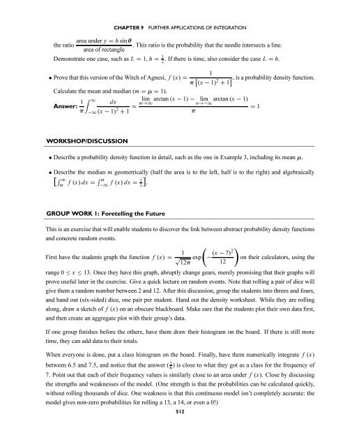
9 FURTHER APPLICATIONS OF INTEGRATION

CHAPTER 9
FURTHER APPLICATIONS OF INTEGRATION
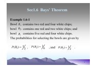
area under y = h sin θ
the ratio . This ratio is the probability that the needle intersects a line.
area of rectangle
Demonstrate one case, such as L = 1, h = 1 2
. If there is time, also consider the case L = h.
1
• Prove that this version of the Witch of Agnesi, f (x) =
π [ (x − 1) 2 ], is a probability density function.
+ 1
Calculate the mean and median (m = μ = 1).
Answer: 1 ∫ ∞
dx
lim arctan (x − 1) − lim arctan (x − 1)
π (x − 1) 2 + 1 = m→∞ n→−∞
= 1
π
−∞
WORKSHOP/DISCUSSION
• Describe a probability density function in detail, such as the one in Example 3, including its mean μ.
• Describe the median m geometrically (half the area is to the left, half is to the right) and algebraically
[ ∫ ∞
m
f (x) dx = ∫ m
−∞ f (x) dx = 1 2].
GROUP WORK 1: Foretelling the Future
This is an exercise that will enable students to discover the link between abstract probability density functions
and concrete random events.
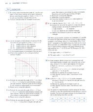
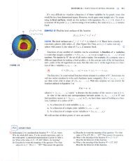
First have the students graph the function f (x) = √ 1
( )
(x − 7)2
exp − on their calculators, using the
12π 12
range 0 ≤ x ≤ 13. Once they have this graph, abruptly change gears, merely promising that their graphs will
prove useful later in the exercise. Give a quick lecture on random events. Note that rolling a pair of dice will
give them a random number between 2 and 12. After this discussion, group the students into threes and fours,
and hand out (six-sided) dice, one pair per student. Hand out the density worksheet. While they are rolling
along, draw a sketch of f (x) on an obscure blackboard. Make sure that the students plot their own data first,
and then create an aggregate plot with their group’s data.
If one group finishes before the others, have them draw their histogram on the board. If there is still more
time, they can add data to their totals.
When everyone is done, put a class histogram on the board. Finally, have them numerically integrate f (x)
between 6.5 and 7.5, and notice that the answer ( 1 6
) is close to what they got as a class for the frequency of
7. Point out that each of their frequency values is similarly close to an area under f (x). Close by discussing
the strengths and weaknesses of the model. (One strength is that the probabilities can be calculated quickly,
without rolling thousands of dice. One weakness is that this continuous model isn’t completely accurate: the
model gives non-zero probabilities for rolling a 13, a 14, or even a 0!)
512